Background
MADS is a derivative-free optimization method supported by global convergence properties where it converges to a minimizer regardless of the starting point. The algorithm consists of two steps as shown in Fig. 1. The first step is an optional search step where the user can run a DOE study or a global optimization study, i.e., genetic algorithm (GA), on a set of variables with size \(n\). The second step is a mandatory local search step called poll-step where the \(2n\) orthogonal poll directions spin around the incumbent solution on the discretized poll frame to randomly choose \(2n\) contiguous directions where the blackbox functions are evaluated on the delimited region containing the poll point.
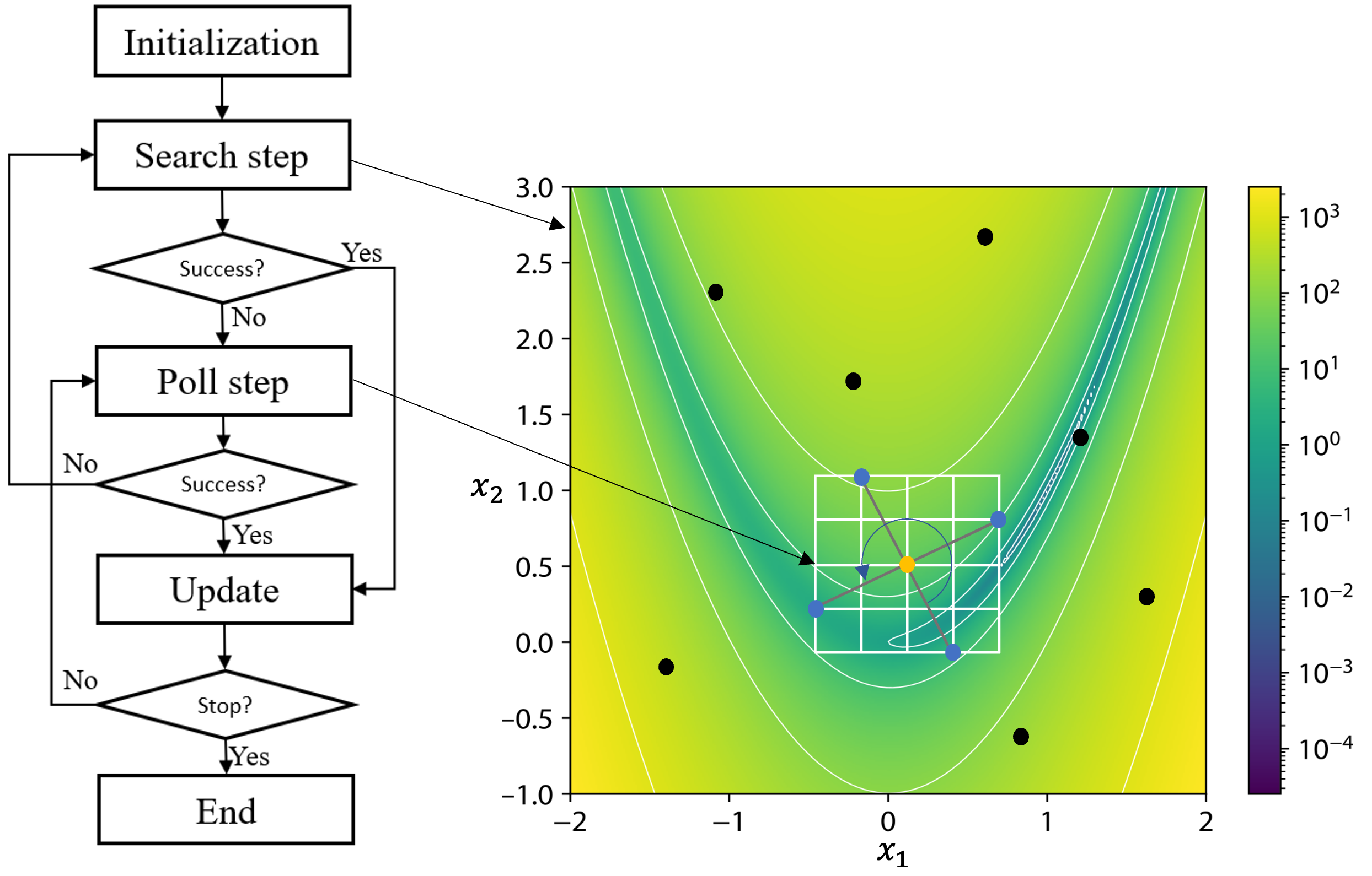
Fig. 1 OMADS flow chart.
When to use OMADS
If the optimization problem is deterministic, then the following checklist will help you to decide whether using OMADS is a recommended choice from a computational speed perspective.
If the optimization problem has a known structure where derivatives are explicit, then exploit them by using an appropriate gradient-based method, i.e., SQP.
If the problem has unknown derivatives, but they can be reliably approximated and the design space has no differentiability issues, then apply an appropriate gradient-based method that supports a model-based algorithm, i.e., NLPQLP.
If the problem has unknown derivatives but can be approximated and the design space has differentiability issues, then apply a derivative-free method that supports model-based algorithms, i.e., COBYLA.
If none of the above works, then use blackbox optimization methods like MADS.
Introduction
In this section, we present the MADS algorithm. We begin with the following definitions of the mesh and the frame from [1, 5]:
Definition: Mesh and Mesh Size Parameter
Let \(G \in \mathbb{R}^{n\times n}\) be an invertible matrix and the columns of \(Z \in \mathbb{Z}^{n \times p}\) form a positive spanning set for \(\mathbb{R}^n\). Define \(D = GZ\). The mesh of coarseness \(\delta^{k} > 0\) generated by \(D\), centered at the incumbent solution \(x_{k} ∈ \mathbb{R}^n\), is defined by \(M^{k} := \{ x^{k} + \delta^{k}D_{y} : y \in \mathbb{N}^{p} \subset \mathbb{R}^{n}, \}\) where \(\delta^{k}\) is called the mesh size parameter.
What distinguishes MADS from the global pattern search (GPS) algorithm is the idea of creating a new parameter, the frame size parameter \(\Delta^{k}\), that replaces \(\delta^{k}\) in the poll step. The frame size parameter \(\Delta^{k}\) defines the frame in which polling is done – polling directions spin around the incumbent solution. At every iteration, these two parameters will satisfy \(0 < \delta^{k} ≤ \Delta^{k}\).
Definition: Frame and Frame Size Parameter
Let \(G \in \mathbb{R}^{n\times n}\) be an invertible matrix and the columns of \(Z \in \mathbb{Z}^{n \times p}\) form a positive spanning set for \(\mathbb{R}^n\). Define \(D = GZ\). Select a mesh size parameter \(\delta^{k} > 0\) and let \(\Delta^{k}\) be such that \(\delta^{k} \leq \Delta^{k}\). The frame of extent \(\Delta^{k}\) generated by \(D\), centered at the incumbent solution \(x_{k} ∈ \mathbb{R}^n\), is defined by \(F^{k} := \{ x \in M^{k} : ||x-x^{k}||_{\infty} \leq \Delta^{k}b \}\) with \(b = \text{max}\{ ||d^{\prime}||_{\infty} : d^{\prime} \in \mathbb{D} \}\) and \(\Delta^{k}\) is called the frame size parameter.
In the MADS algorithm, the poll set is constructed by selecting mesh points from inside the frame \(F_{k}\), and is not necessarily forced to equal \(P_{k}\). By having the mesh size parameter decrease more rapidly than the frame size parameter, this allows for asymptotically dense selections of poll directions, see Fig. 2.
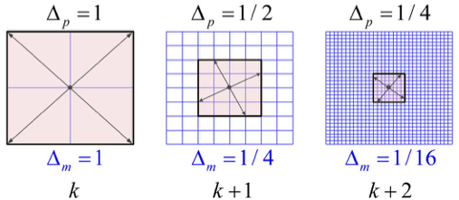
Fig. 2 Mesh and poll updates.
MADS algorithm
In this section, we will demonstrate how each step of the MADS algorithm, shown in Algorithm 1, works and how they are implemented in OMADS.
             % This quicksort algorithm is extracted from Chapter 7, Introduction to Algorithms (3rd edition)
 \begin{algorithm}
 \caption{Mesh adaptive direct search (MADS)}
 \begin{algorithmic}
 \STATE{Given $f : \mathbb{R}^{n} \mapsto  \mathbb{R} \cup \{ \infty \}$ and a starting point $x^{0} \in \Omega$ and barrier function $f_{\Omega}(x)$}
 \PROCEDURE{Initialization}{}
     \STATE{$\Delta^{0} \in (0, \infty)$} initial frame size
     \STATE{$D=GZ$} positive spanning matrix
     \STATE{$\tau \in (0,1)$, with $\tau$ rational} mesh size adjustment parameter
     \STATE{$\epsilon_{\text{stop}} \in [0,\infty)$} stopping tolerance
     \STATE{$k \gets 0$}  iteration counter
 \ENDPROCEDURE
 \PROCEDURE{Update}{}
     \STATE{set the mesh size parameter to $\delta^{k} = \text{min} \{ \Delta^{k}, (\Delta^{k})^{2} \}$}
 \ENDPROCEDURE
 \PROCEDURE{Search}{}
     \IF{$f_{\Omega}(t) < f_{\Omega}(x^{k})$ for some t in a finite subset $S^{k}$ of $M^{k}$}
         \STATE set $x^{k+1} \gets t$ and $\Delta^{k+1} \gets \tau^{-1} \Delta^{k}$ and go to 27
     \ELSE
         \STATE go to 19
     \ENDIF
 \ENDPROCEDURE
 \PROCEDURE{Poll}{}
     \STATE select a positive spanning set $\mathbb{D^{k}_{\Delta}}$ such that \\
     $P^{k}=\{x^{k}+\delta^{k}:d\in\mathbb{D}^{k}_{\Delta}\}$ \\
     is a subset of the frame $F^{k}$ of extent $\Delta^{k}$
     \IF{$f_{\Omega}(t) < f_{\Omega}(x^{k})$ for some $t$ in $t \in P^{k}$}
         \STATE set $x^{k+1} \gets t$ and $\Delta^{k+1} \gets \tau^{-1} \Delta^{k}$
     \ELSE
         \STATE set $x^{k+1} \gets x^{k}$ and $\Delta^{k+1} \gets \tau \Delta^{k}$
     \ENDIF
 \ENDPROCEDURE
 \PROCEDURE{Terminate}{}
     \IF{$\Delta^{k+1}\geq \epsilon_{stop}$}
         \STATE increament $k \gets k+1$ and go to 9
     \ELSE
         \STATE stop
     \ENDIF
 \ENDPROCEDURE
 \end{algorithmic}
 \end{algorithm}
Initialization step
In this step, we can set the initial frame size \(\Delta_{0}\), generate the initial positive spanning set matrix \(D_{0}\), adjust the initial mesh size and set the termination criteria before firing up the study.
Let us see how we can do that in OMADS. The class responsible for MADS preprocessing is called ‘PreMADS’ which uses the data dictionaries that hold user inputs required to initialize the algorithm:
""" Run preprocessor for the setup of
 the optimization problem and the initialization
of optimization process """
iteration, xmin, poll, options, param, post, out = PreMADS(data).initialize_from_dict()
The data dictionary consists of four other dictionaries:
Evaluator settings which have the following five keys:
blackbox: The name of the callable or executable fileinternal: Specify whether the evaluator is a callable function, a blackbox executable file, or an internal benchmarking testInternal takes one of these values:
uncon: Unconstrained benchmarkingcon: Constrained benchmarkingexe: Executable blackbox
path: The evaluation path that should contain the executable file (if any)input: For the case of blackbox executables, it is the input file required to run the blackboxoutput: For the case of blackbox executables, it is the output file that will be parsed to extract response outputs
Example:
"evaluator":
  {
    "blackbox": "rosenbrock",
    "internal": "uncon",
    "path": "./bm",
    "input": "input.inp",
    "output": "output.out"}
If the evaluator is a callable function, the blackbox key has to be assigned to the callable function name, but no need to define other keys under the evaluator dictionary, see the following example.
eval = {"blackbox": fun}
Note
For blackbox files, the input file should contain one column that has the design vector values that follow the same order as the variables populated in the global design vector. The output file should hold all the evaluated response outputs where the first value in the vector will be assigned to the objective function and the other values will be assigned to the constraint functions, respectively.
Parameter settings that have the following keys:
name: Run name (important for saving the output files in the post directory. If not specified the output folder will be named asunknown)baseline: The design initial pointlb: Lower boundub: Upper boundvar_names: Variables namevar_types: Variables type *R: Continuous variable (real value) *I: Integer variable *C_<set name>: Categorical variable. A set name from the sets dictionary should be added after the underscore that follows the C *D_<set name>: Discrete variable. A set name from the sets dictionary should be added after the underscore that followsDSets: a dictionary where its keys refer to the set name and their value should be assigned to a list of values (the values can be of heterogeneous type)scaling: The scaling factorpost_dir: The post directoryconstraints_type: List of the constraints barrier type *PB: Progressive barrier *EB: Extreme barrierLAMBDA: List of the initial Lagrangian multipliers value assigned to the constraintsRHO: List of the initial penalty parameterhmax: The maximum feasibility threshold
Example:
"param":
  {
    "name": "pressure_vessel",
    "baseline": [99, 99, 50, 200],
    "lb": [1, 1, 10, 10],
    "ub": [99,99,200, 200],
    "var_names": ["x1", "x2", "x3", "x4"],
    "scaling": [98,98,190,190],
    "constraints_type": ["PB", "EB", "PB", "PB"],
    "LAMBDA": [5, 5, 5, 5],
    "RHO": 0.0001,
    "post_dir": "./tests/bm/constrained/post",
    "h_max": 1
  },
Search step options dictionary which has the following keys: *
search: The search step options *type: Search type can take one of the following valuesVNS: Variable neighbor searchsampling: Sampling searchBO: Bayesian optimization (TODO: not published yet as it is still in the testing and BM phase)NM: Nelder-Mead (TODO: not published yet as it is still in the testing and BM phase)PSO: Particle swarm optimization (TODO: not published yet as it is in the testing phase)CMA-ES: Covariance matrix adaptation evolution strategy (TODO: not published yet as it is in the testing phase)
s_method: Can take one of the following values *LH: Latin Hypercube sampling*RS: Random sampling *HALTON: Halton samplingns: Number of samples
Example:
"search": {
    "type": "VNS",
    "s_method": "LH",
    "ns": 100
  }
Algorithmic options dictionary which has the following keys:
seed: The random generator seed that ensures results reproducibility. This should be an integer valuebudget: The evaluation budget; the maximum number of evaluations for the blackbox definedtol: The minimum poll size tolerance; the algorithm terminates once the poll size falls below this valuepsize_init: Initial poll sizedisplay: A boolean for displaying verbose outputs per iteration in the terminal windowopportunistic: A boolean for enabling an opportunistic searchcheck_cache: A boolean for checking if the current point is a duplicate by checking its hashed address (integer signature)store_cache: A boolean for saving evaluated designs in the cache memorycollect_y: Currently inactive (to be used when the code is integrated with the PyADMM MDO module)rich_direction: A boolean that enables capturing a rich set of directions in a generalized patternprecision: A string character input that controls the dtype decimal resolution used by the numerical library numpyhigh: float128 1e-18medium: float64 1e-15low: float32 1e-8
save_results: A boolean for generating a MADS.csv file for the output results under the post directorysave_coordinates: Saving poll coordinates (spinners) of each iteration in a JASON dictionary template that can be used for visualizationsave_all_best: A boolean for saving only incumbent solutionsparallel_mode: A boolean for parallel computation of the poll set
Example:
"options":
  {
    "seed": 0,
    "budget": 10000,
    "tol": 1e-12,
    "psize_init": 1,
    "display": true,
    "opportunistic": false,
    "check_cache": true,
    "store_cache": true,
    "collect_y": false,
    "rich_direction": true,
    "precision": "high",
    "save_results": false,
    "save_coordinates": false,
    "save_all_best": false,
    "parallel_mode": false,
    "np": 4
  }
Update parameters
After checking the termination criteria, the mesh parameters update step can be called by reaching that step all the running serial/parallel processes are supposed to be done. It is important to ensure that poll directions have been evaluated on the same mesh and frame parameters, particularly in parallel points evaluation.
This is the code used to update the poll and mesh parameters:
def master_updates(self, x: List[Point], peval):
  if peval >= self.eval_budget:
    self.terminate = True
  for xtry in x:
    """ Check success conditions """
    if xtry < self.xmin:
      self.success = True
      self.nb_success += 1
      """ Update the post instant """
      del self._xmin
      self._xmin = Point()
      self._xmin = copy.deepcopy(xtry)
      if self.display:
        if self._dtype.dtype == np.float64:
          print(f"Success: fmin = {self.xmin.f:.15f} (hmin = {self.xmin.h:.15})")
        elif self._dtype.dtype == np.float32:
          print(f"Success: fmin = {self.xmin.f:.6f} (hmin = {self.xmin.h:.6})")
        else:
          print(f"Success: fmin = {self.xmin.f:.18f} (hmin = {self.xmin.h:.18})")

      self.mesh.psize_success = copy.deepcopy(self.mesh.psize)
      self.mesh.psize_max = copy.deepcopy(maximum(self.mesh.psize,
                            self.mesh.psize_max,
                            dtype=self._dtype.dtype))
Note
The update function belongs to the poll class. The method is named master_update to refer to the master process in the parallel-space decomposition which will be included in future versions of OMADS.
Search step
This step breaks free of local minimizers, and it is restricted to the mesh. The search step is discussed in more details in the documentation of StatML and RAF that can be found in [4, 6].
Poll step
The MADS algorithm is permitted to select any poll direction such that \(x^{k}+\delta^{k}d\) lies inside the frame where \(\delta^{k}d \leq \Delta^{k}b\) for all \(d \in \mathbb{D}^{k}_{\Delta}\). Since \(\Delta^{k}>\delta^{k}\) whenever \(\delta^{k} < 1\) which provides flexibility in how the poll set is constructed.
We will give here a glimpse of the MADS convergence properties and the meaning of the dense sets (richness) of poll directions. In MADS, any direction that is sampled in the limit of a refining sequence must have a nonnegative directional derivative. Moreover, the directions are generated from an ever-expanding set of options where the mesh size parameter \(\delta_{k}\) goes to zero more rapidly than the poll size parameter \(\Delta_{k}\).
MADS can produce an asymptotically dense set of poll directions that can be demonstrated by using the Householder matrix. Firstly, let’s define the dense subset
Definition: Asymptotically Dense
The set \(V \subseteq \mathbb{R}^{n}\) is said to be asymptotically dense if the normalised \(set \{v/||v||:v \in V\}\) is dense on the unit sphere \(S=\{w\in \mathbb{R}^{n} :|w|= 1\}\).
Now the Householder matrix can be defined as:
Definition: Householder Matrix
Let \(V \subseteq \mathbb{R}^{n}\) be a normalized vector. The Householder matrix H associated with \(v\) is \(H:=I-2vv^{T} \in \mathbb{R}^{n \times n}\), where I is the \(n \times n\) identity matrix.
Let \(v\) be a nonzero in \(\mathbb{R}^{n}\) and \(H\) be the associated Householder matrix. Then for any \(\gamma H [ I-I ]\) forms a maximal positive basis of \(\mathbb{R}^{n}\).
             \begin{algorithm}
 \caption{Creating the set of poll directions}
 \begin{algorithmic}
 \PROCEDURE{Create-Householder-matrix}{}
     \STATE{use $v_{k}$ to create its associated Householder matrix}
     \STATE{$H^{k} = [h_{1} \, h_{2} \, ..., \, h_{n}]$}
 \ENDPROCEDURE
 \PROCEDURE{Create-poll-set}{}
     \STATE{define $\mathbb{B}^{k} = \{b1,b2, ..., b_{n}\}$ with $b_{j}=\text{round}(\frac{\Delta_{k}}{\delta{k}}\frac{h_{j}}{||h_{j}||_{\infty}})$}
     \STATE{set $\mathbb{D}^{k}_{\Delta} = \mathbb{B}^{k} \cup (-\mathbb{B}^{k})$ }
 \ENDPROCEDURE

 \end{algorithmic}
 \end{algorithm}
In OMADS, Algorithm 2 is implemented under the directions class Dirs2n in a function called create_housholder.
def create_housholder(self, is_rich: bool) -> np.ndarray:
  """Create householder matrix

  :param is_rich:  A flag that indicates if the rich direction option is enabled
  :type is_rich: bool
  :return: The householder matrix
  :rtype: np.ndarray
  """
  hhm: np.ndarray
  if is_rich:
    v_dir = copy.deepcopy(self.ran())
    v_dir_array = np.array(v_dir, dtype=self._dtype.dtype)
    v_dir_array = np.divide(v_dir_array,
                (np.linalg.norm(v_dir_array,
                        2).astype(dtype=self._dtype.dtype)),
                dtype=self._dtype.dtype)
    hhm = np.subtract(np.eye(self.dim, dtype=self._dtype.dtype),
              np.multiply(2.0, np.outer(v_dir_array, v_dir_array.T),
                    dtype=self._dtype.dtype),
              dtype=self._dtype.dtype)
  else:
    hhm = np.eye(self.dim, dtype=self._dtype.dtype)
  hhm = np.dot(hhm, np.diag((np.abs(hhm, dtype=self._dtype.dtype)).max(1) ** (-1)))
  # Rounding( and transpose)
  tmp = np.multiply(self.mesh.rho, hhm, dtype=self._dtype.dtype)
  hhm = np.transpose(np.multiply(self.mesh.msize, np.ceil(tmp), dtype=self._dtype.dtype))
  hhm = np.dot(np.vstack((hhm, -hhm)), self.scaling)

  return hhm
Then the generated Householder matrix will be used in the following function to create the poll set:
def create_poll_set(self, hhm: np.ndarray, ub: List[float], lb: List[float], it: int):
  """Create the poll directions

  :param hhm: Householder matrix
  :type hhm: np.ndarray
  :param ub: Variables upper bound
  :type ub: List[float]
  :param lb: Variables lower bound
  :type lb: List[float]
  :param it: iteration
  :type it: int
  """
  del self.poll_dirs
  temp = np.add(hhm, np.array(self.xmin.coordinates), dtype=self._dtype.dtype)
  # np.random.seed(self._seed)
  temp = np.random.permutation(temp)
  temp = np.minimum(temp, ub, dtype=self._dtype.dtype)
  temp = np.maximum(temp, lb, dtype=self._dtype.dtype)

  for k in range(2 * self.dim):
    tmp = Point()
    tmp.coordinates = temp[k]
    tmp.dtype.precision = self.dtype.precision
    self.poll_dirs = tmp
    del tmp
  del temp

  self.iter = it
F3 depicts the dense directions on the same frame size where
We recommend you to visit [5] for further details on the proofs of Householder positive basis that show how the columns of the associated Householder matrices are asymptotically dense, given a dense set of directions in the unit sphere S.
Termination
Typically, the algorithm terminates when the evaluation budget is exhausted and/or the poll size falls below the tolerance size.