Benchmarking

This section describes how OMADS 2610 is benchmarked: the regression suite that runs on every commit, and the COCO bbob-constrained runner for large studies.

Regression suite

tests/test_OMADS_BASIC.py runs on Linux, Windows and macOS in continuous integration. Every solver must reach a target value within a fixed budget. For the 10D and 20D Rosenbrock problems, the target is the median over three seeds (single-seed results swing too much with the random direction stream).

Problem	\(n\)	Budget	Solver: target
Rosenbrock, \(x^0 = (-2.5, \dots)\)	2	3500	mads ≤ 0.005, poll ≤ 0.008, search ≤ 0.07
Thin constrained band (2 PB constraints)	2	2000	mads ≤ 0.0989
Rosenbrock (ORTHO N+1)	10	4000 / 3000	mads ≤ 9.7, poll ≤ 8, search ≤ 7.3
Rosenbrock (ORTHO N+1)	20	5000	mads ≤ 20.5, poll ≤ 20, search ≤ 24.3
Geometric programming (6 PB constraints)	10	10000	poll ≤ 27 (median)
Sellar, IDF formulation (GMESH)	4	150	runs to completion

The 2D Rosenbrock test also runs every solver in parallel mode (np = 4) and checks the same targets.

Run the suite locally with:

$ pip install -e ".[test]"
$ pytest tests -v

COCO bbob-constrained

benchmarks/coco/run_mads_bbob_constrained.py runs mads.main on the 54 functions of the COCO bbob-constrained suite [Hansen et al., 2021]. Each COCO problem \(x \mapsto f(x)\) with constraints \(g(x) \le 0\) becomes a callable blackbox returning [f, g], and every constraint uses the progressive barrier. A run stops as soon as COCO’s final target is hit, and unsolved instances are restarted (new start point and seed) until budget_multiplier × dimension evaluations are used.

The runner’s defaults are the configuration published below (--preset A): the ACTIVE sampling search with \(n_s = \min\{(n+1)(n+2)/2,\ 2n\}\), the ORTHO_N+1 poll and opportunistic evaluation, on dimensions 2, 3, 5 and 10, instances 1 to 15, with a budget of \(100\,n\). The other published configurations are available as presets, and any option overrides its preset value.

$ pip install -r benchmarks/coco/requirements.txt
$ python benchmarks/coco/run_mads_bbob_constrained.py                  # preset A
$ python benchmarks/coco/run_mads_bbob_constrained.py --preset halton
$ python benchmarks/coco/run_mads_bbob_constrained.py -d 2,3,5 -f 1-12 -i 1-3 \
      --budget-multiplier 50

Results go to exdata/<output-folder> and are post-processed with cocopp into an HTML report under ppdata/. Large runs can be split over several processes with --batches N --batch k; post-process all the batch folders together with python -m cocopp exdata/....

Table 1 Presets of the COCO runner

Preset	COCO name	Configuration
A (default)	OMADS-A	ACTIVE search, \(n_s = \min\{(n+1)(n+2)/2,\ 2n\}\), ORTHO_N+1 poll, opportunistic.
B	OMADS-B	ACTIVE search, \(n_s = (n+1)(n+2)/2\), after every third failed poll, ORTHO_N+1 poll, opportunistic.
halton	OMADS-Halton	HALTON search, \(n_s = 1\) (56 on f43 to f54), ORTHO_2N poll.
initial	OMADS-ACTIVE	ACTIVE search, \(n_s = (n+1)(n+2)/2 + 10\), ORTHO_2N poll.

Table 2 Main options of the COCO runner

Option	Default	Meaning
--preset	A	Published configuration (see the table above).
--budget-multiplier, -b	100	Evaluations per instance, times the dimension.
--dimensions, -d	2,3,5,10	Dimensions to run (the suite has 2, 3, 5, 10, 20, 40).
--functions, -f	all	Function indices, e.g. 1-18 (1 to 54).
--instances, -i	1-15	Instance indices.
--s-method	preset	Sampling method of the search step (ACTIVE, HALTON, LH, …).
--ns / --ns-multimodal	preset	Samples per search step on f1 to f42 and on the multimodal Rastrigin functions f43 to f54: an integer, quad for \((n+1)(n+2)/2\), min2n for \(\min\{(n+1)(n+2)/2,\ 2n\}\) or auto for \((n+1)(n+2)/2 + 10\).
--search-every	preset	Run the sampling search after every k-th consecutive failed poll only.
--direction-type	preset	Poll directions: ORTHO_2N or ORTHO_N+1.
--opportunistic / --no-opportunistic	preset	Stop evaluating a poll or search set at its first improvement.
--mesh-type	GMESH	GMESH (anisotropic granular mesh) or ORTHO.
--anisotropy-factor	0.05	GMESH anisotropy factor.
--min-mesh-size	1e-13	GMESH minimum mesh size.
--seed	1234	Base seed, offset at each restart.
--batches, --batch	1, 1	Split the suite and pick the batch run by this process.

Results on bbob-constrained

Experimental setup

OMADS 2610 was run on the 54 functions of bbob-constrained in dimensions 2, 3, 5 and 10, on instances 1 to 15, with a budget of \(100\,n\) function evaluations per instance (810 runs per dimension). All runs use mads.main with the settings of the COCO runner (granular mesh, progressive barrier on every constraint). The quadratic model search runs first at every iteration in all configurations; they differ in the sampling search and the poll.

Label	Configuration
ACTIVE (A)	"s_method": "ACTIVE" (BiTPE) with smaller batches, \(n_s = \min\{(n+1)(n+2)/2,\ 2n\}\) (4, 6, 10 and 20 in dimensions 2, 3, 5 and 10); ORTHO_N+1 poll; "opportunistic": True.
ACTIVE (B)	"s_method": "ACTIVE" (BiTPE) with \(n_s = (n+1)(n+2)/2\), run only after every third consecutive unsuccessful poll ("search_every": 3); ORTHO_N+1 poll; "opportunistic": True.
HALTON	"s_method": "HALTON", \(n_s = 1\) (\(n_s = 56\) on the multimodal functions f43 to f54); ORTHO_2N poll; the default of the COCO runner.
ACTIVE, ns = (n+1)(n+2)/2 + 10	"s_method": "ACTIVE" with \(n_s = (n+1)(n+2)/2 + 10\) after every unsuccessful poll; ORTHO_2N poll. A first configuration, reported in Table 3 only.

With the ACTIVE search, each model-based search step evaluates up to \(n_s\) BiTPE proposals plus three line probes (the runner sets search["batch"] to \(n_s\); OMADS’ default is 10); with "opportunistic": True the evaluation of a poll or search set stops at its first improvement.

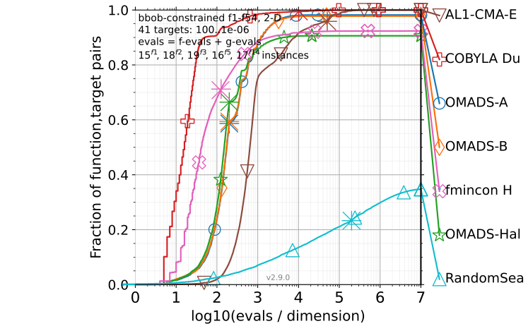
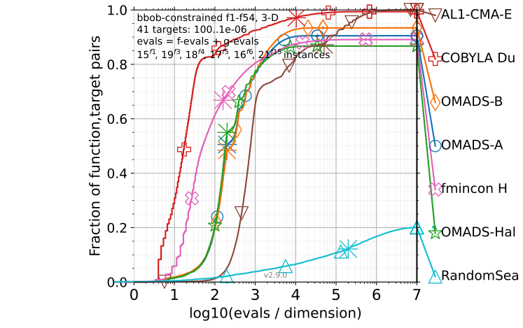
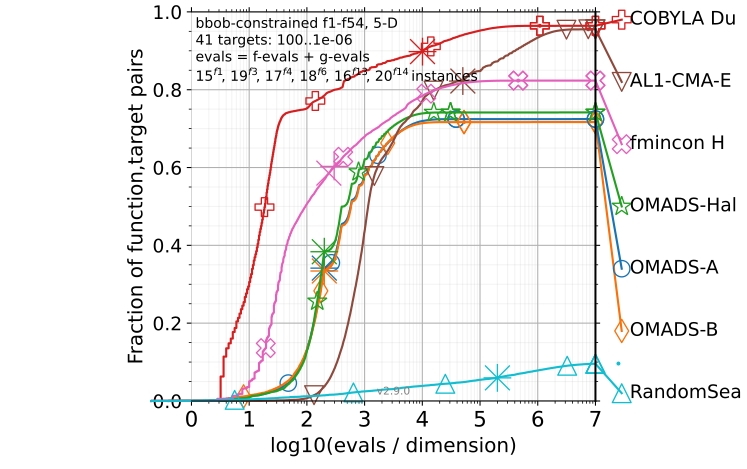
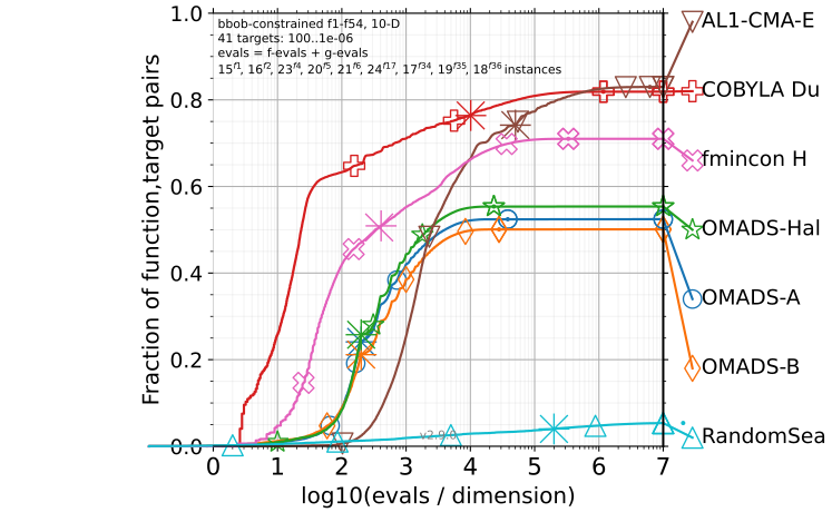
The reference algorithms are the 2022 entries of the COCO data archive: COBYLA and AL1-CMA-ES (Dufossé), fmincon (Hellwig) and random search. These were run with much larger budgets, up to \(10^{7}\,n\) evaluations. Note that COCO counts every constraint evaluation in addition to the objective evaluation (“evals = f-evals + g-evals”), which is why the OMADS curves extend beyond \(\log_{10}(100) = 2\) on the horizontal axis.

Fraction of solved runs

Figure 4 and Table 3 report, for each configuration and dimension, the fraction of the 810 runs whose final precision \(f - f_{\text{opt}}\) reached \(10^{-1}\), \(10^{-3}\) and \(10^{-6}\) within the budget.

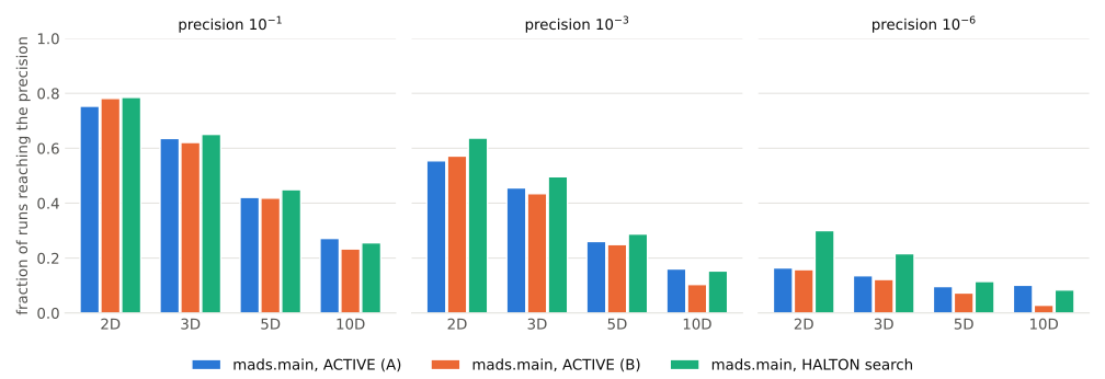
Figure 4 Fraction of bbob-constrained runs (54 functions × 15 instances) reaching a given precision within \(100\,n\) evaluations, for three configurations of mads.main.

Table 3 Fraction of runs reaching each precision (data of Figure 4).

algorithm	dimension	runs	reached 0.1	reached 0.001	reached 1e-06
mads.main, ACTIVE (A)	2	810	0.753	0.554	0.164
mads.main, ACTIVE (A)	3	810	0.636	0.456	0.136
mads.main, ACTIVE (A)	5	810	0.421	0.260	0.096
mads.main, ACTIVE (A)	10	810	0.272	0.160	0.101
mads.main, ACTIVE (B)	2	810	0.781	0.572	0.158
mads.main, ACTIVE (B)	3	810	0.621	0.435	0.122
mads.main, ACTIVE (B)	5	810	0.419	0.249	0.073
mads.main, ACTIVE (B)	10	810	0.233	0.104	0.028
mads.main, HALTON search	2	810	0.785	0.637	0.300
mads.main, HALTON search	3	810	0.651	0.496	0.216
mads.main, HALTON search	5	810	0.449	0.288	0.115
mads.main, HALTON search	10	810	0.256	0.153	0.084
mads.main, ACTIVE, ns = (n+1)(n+2)/2 + 10	2	810	0.093	0.005	0.000
mads.main, ACTIVE, ns = (n+1)(n+2)/2 + 10	3	810	0.088	0.010	0.000
mads.main, ACTIVE, ns = (n+1)(n+2)/2 + 10	5	810	0.025	0.001	0.000
mads.main, ACTIVE, ns = (n+1)(n+2)/2 + 10	10	810	0.015	0.002	0.000

Runtime distributions

The grid in Table 4 shows the empirical cumulative distribution functions (ECDFs) of the runtime, aggregated over all 54 functions, as produced by cocopp. Each curve gives the fraction of (function, target) pairs, for 41 targets between \(10^{2}\) and \(10^{-6}\), solved after a given number of evaluations divided by the dimension. In the legends, OMADS-A, OMADS-B and OMADS-Hal stand for ACTIVE (A), ACTIVE (B) and HALTON (cocopp truncates the labels).

Table 4 Runtime ECDFs aggregated over all bbob-constrained functions, in 2, 3, 5 and 10 dimensions.

Discussion

• The cost of the ACTIVE search decides its usefulness at this budget. With \(n_s = (n+1)(n+2)/2 + 10\) after every unsuccessful poll, a search step costs up to \(79\) of the \(1000\) evaluations available in dimension 10, and fewer than 10% of the runs reach \(10^{-1}\) in any dimension. Capping the batch at \(2n\) (ACTIVE (A)), or running the search after every third failed poll only (ACTIVE (B)), together with the cheaper ORTHO_N+1 poll and opportunistic evaluation, brings the ACTIVE search level with the HALTON configuration.

• In dimension 10, ACTIVE (A) is the best configuration at every precision: 27.2% of the runs reach \(10^{-1}\) (25.6% for HALTON), 16.0% reach \(10^{-3}\) (15.3%) and 10.1% reach \(10^{-6}\) (8.4%). In dimension 5 the two ACTIVE configurations are within three points of HALTON.

• In dimensions 2 and 3, HALTON remains ahead, mostly at tight precisions; there the one-point sampling search leaves almost the whole budget to the model search and the poll.

• The runtime distributions (Table 4) give a complementary view, over 41 targets instead of three precisions. In dimension 2, both ACTIVE configurations solve about 98% of the (function, target) pairs within their budget, more than HALTON (91%) and fmincon (92%), and close to COBYLA and AL1-CMA-ES, which use up to \(10^{7}\,n\) evaluations. In dimension 10, HALTON solves slightly more pairs (55%) than ACTIVE (A) (52%) and ACTIVE (B) (50%): it reaches more of the easy targets, while ACTIVE (A) reaches more of the tight ones.

• Smaller batches generalize better than a less frequent search: ACTIVE (B), which keeps the large batches, is close to ACTIVE (A) in dimensions 2 to 5 but falls behind in dimension 10.

• COBYLA and fmincon, two model-based local solvers, are faster on these constrained, mostly smooth functions; they also reach more targets because they were run with budgets several orders of magnitude larger.

Results reproducibility

The results above are reproduced, from the benchmark runs to the figures and the table of this page, by a single script.

Requirements. Python 3.10 or newer and an internet connection (cocopp downloads the reference algorithms from the COCO data archive on first use). From the root of the OMADS repository, install OMADS and the benchmarking packages (coco-experiment, cocopp and matplotlib):

$ python -m pip install -e .
$ python -m pip install -r benchmarks/coco/requirements.txt

Run.

$ python benchmarks/coco/reproduce_results.py

The script

1. runs the four presets A, B, halton and initial of run_mads_bbob_constrained.py on dimensions 2, 3, 5 and 10, instances 1 to 15, with a budget of \(100\,n\), each split into 12 batches executed in parallel (a batch that fails is run again once);

2. gathers the batches of each preset into exdata/OMADS-A, exdata/OMADS-B, exdata/OMADS-Halton and exdata/OMADS-ACTIVE;

3. post-processes OMADS-A, OMADS-B and OMADS-Halton with cocopp against COBYLA, AL1-CMA-ES, fmincon and random search (full HTML report in ppdata/repro);

4. writes the runtime ECDFs (Table 4) and, from all four presets, the summary chart and table (Figure 4 and Table 3) to docs_src/media/figures/coco. Rebuild the documentation with sphinx-build -b html docs_src docs to update this page.

On a 24-core workstation with 12 parallel processes, the runs take about 8 to 10 hours, most of it for presets A and B in dimension 10, and cocopp about half an hour more.

Table 5 Options of reproduce_results.py

Option	Default	Meaning
--presets	A,B,halton,initial	Presets to run.
--workers	half the CPU cores, at most 12	Parallel processes. On a 64 GB machine, 12 processes run without problems while 24 run out of memory; lower it if batches fail with memory errors.
--batches	12	Batches per preset.
-d, -f, -i	runner defaults	Dimensions, functions and instances, for a reduced reproduction.
--workdir	repository root	Folder that receives exdata/ and ppdata/repro.
--figures	docs_src/media/figures/coco	Where the figures and table are written.
--skip-runs	off	Reuse existing exdata/ data and only post-process.

A single configuration can also be run on its own, for example python benchmarks/coco/run_mads_bbob_constrained.py --preset B, and post-processed with benchmarks/coco/postprocess_bbob_constrained.py and benchmarks/coco/summarize_bbob_constrained.py.

Note

The sampling search draws random numbers that are not all controlled by the run seed, so repeated campaigns give slightly different individual runs. The aggregated fractions and runtime distributions agree to within about one percentage point.

Toy problems

Results on the 2D toy functions, from the Toy problems, with mads.main, seed 0 and a 1000-evaluation budget (2000 for Eggholder):

Function	Global minimum	OMADS fmin	Evaluations	Search
Rosenbrock	0	0.0	223	ACTIVE
Alpine	0	4.5e-06	270	ACTIVE
Ackley 3	−186.4112	−186.4112	253	ACTIVE
Eggholder	−959.6407	−959.6407	871	LH, ns = 30