Background
Engineering systems are often intrinsically decomposable such that they can be developed following a decomposition paradigm. The system decomposed components can be severally developed. This allows optimal system design problem to be decomposed into subproblems, each of which is associated with a system component. Solving these optimization subproblems autonomously requires a coordination scheme to account for systems interaction and to ensure the consistency and optimality of a system-level design.
Fig. 1 Interdisciplinary interactions
Coordination methods used for distributed multidisciplinary design optimization (MDO) include penalty-based decomposition [1, 2], bilevel integrated system synthesis [3, 4], collaborative optimization [5, 6, 7, 8], quasi-separable decomposition [9] and alternating directions method of multipliers (ADMM) [10, 11, 12]. We will focus on the analytical target cascading (ATC) method, which, according to the classification in [13], is an alternating method with closed design constraints and open consistency constraints.
ATC was motivated by translating system-level design targets to design specifications for the subsystems (components) that constitute the system [14, 15]. Design targets are cascaded using a hierarchical problem decomposition such that subproblems, associated with the components of the system, not only determine targets for their children, but also compute responses to targets they receive and communicate these back to their parents, as depicted in Fig. 2. The objective of a subproblem is to minimize the deviations between the target-response pairs while maintaining feasibility with respect to its local design constraints [16].

Fig. 2 Target-response coupling between the parent subproblem \(p_{i}\) and its child subproblem \(p_{j}\).
The conventional ATC formulation uses a hierarchical problem decomposition paradigm to decompose the problem into subproblems. The term hierarchical here refers to the functional dependency among system components; responses of high-level components in the hierarchy depend on responses of low-level components in the hierarchy, but not the converse, see Fig. 3 (a). However, that might won’t work for coordinating subproblems that do not have a hierarchical decomposition structure. For example, MDO problems are often composed of subproblems governed by analyses that have no hierarchical pattern, see Fig. 3 (b). On top of that, the functions of decomposed optimal system design subproblems might depend on variables of more than one subproblem, as shown in Fig. 3 (c). Such coupling functions usually represent a system attribute such as mass, cost, volume, or power. Coordinating system-wide requirements using the hierarchical ATC formulation requires the introduction of at least as many target-response pairs as there are subproblems.
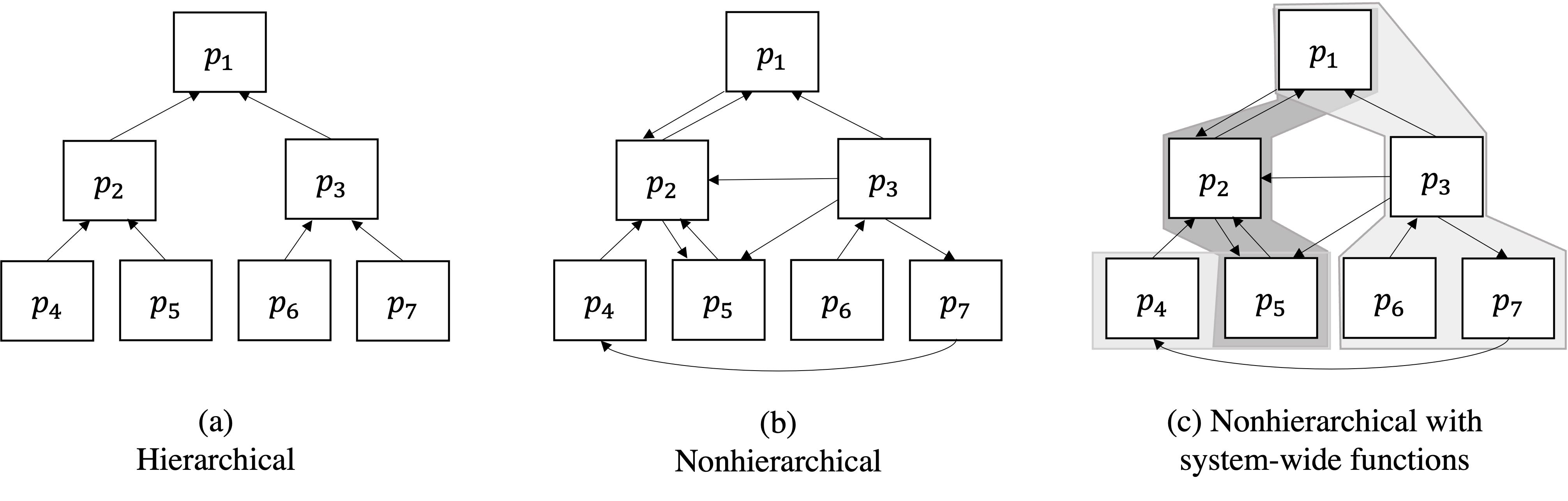
Fig. 3 Functional dependence structure of the original and proposed ATC formulations: The arrows indicate the flow of subproblem responses; the shaded boxes are used to represent the dependence of system-wide functions on subproblem variables.
Nonhierarchical analytical target cascading (NHATC) is an extension to ATC that aims to include nonhierarchical target-response coupling among subproblems so that functional dependencies in nonhierarchical problem decomposition can be handled by the ATC process while preserving the unique target-response coupling structure that distinguishes ATC from other coordination methods.
Introduction
As the complexity of engineering systems grows, the engineering design task becomes more challenging due to distributed design processes that mostly rely on big historical data and/or experts opinion. Multidisciplinary design optimization (MDO) aims at leveraging system’s performance that relies on the evaluated design criteria of several disciplines and processes. MDO is critical to coordinating concurrent analysis and design activities in order to account for and exploit the interactions of multiple physics-based engineering disciplines such as aerodynamics, structures, thermodynamics, etc., as well as the disciplines pertinent to life-cycle aspects. For instance, Fig. 4 shows the coupling relationships among various interacting disciplines in the design process of the supersonic business jet system that includes recursive workflows, which usually don’t converge, and shared design variables.
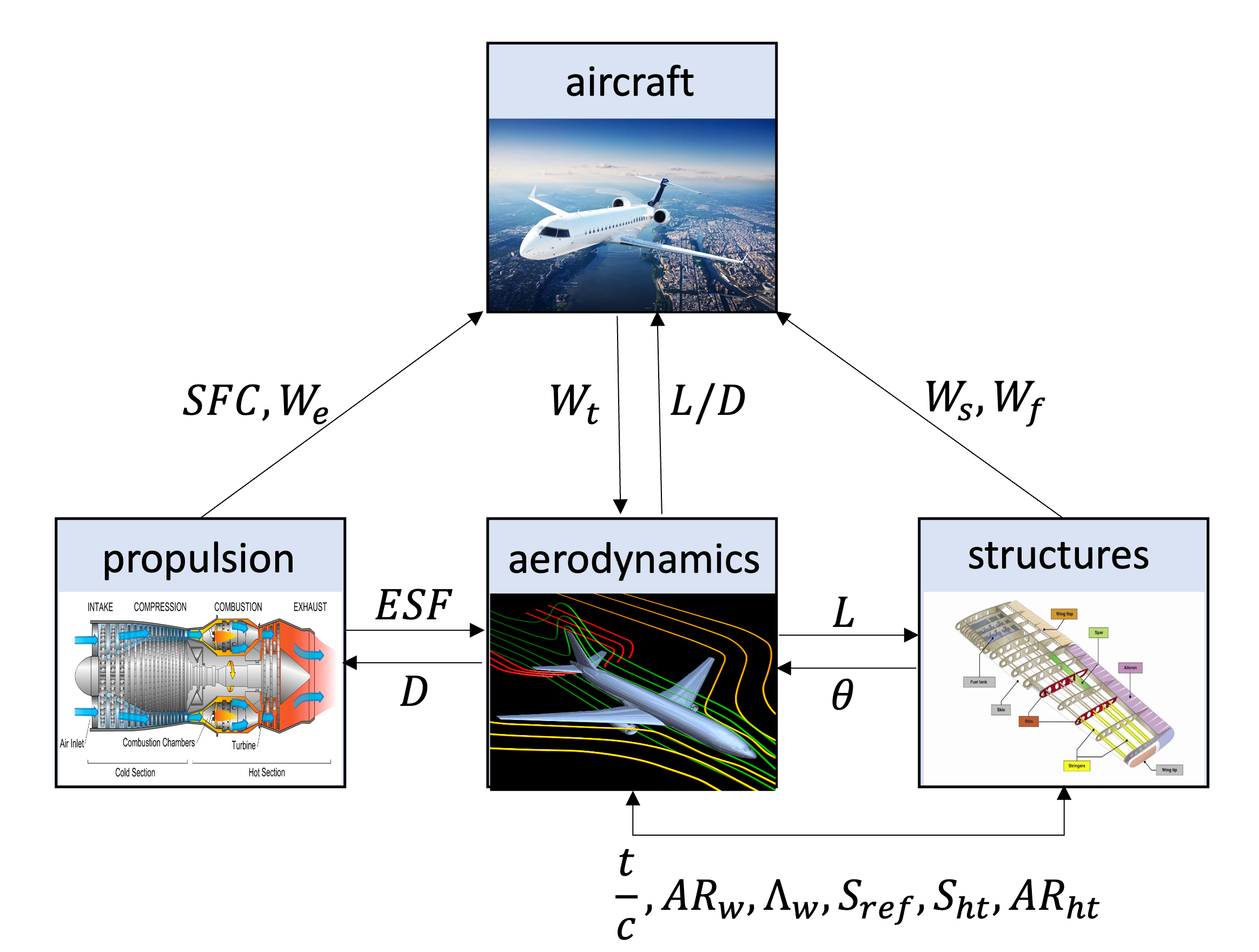
Fig. 4 Data dependencies for business jet problem. Single arrows indicate direction of response flow, and double arrows indicate shared variables.
When to use DMDO
Solving one large MDO problem all-in-one works great if the multidisciplinary (system) analysis (MDA) converges, so the following checklist will help you to decide whether using DMDO is a recommended choice.
For single- and multi-objective studies, use DMDO if you deal with any of the following situations
If the MDA process doesn’t converge (MDA typically does not converge for tightly-coupled systems)
If the optimization algorithm used cannot exploit available disciplinary knowledge (if any)
If the optimization algorithm cannot handle large-diemnsional design space
For multi-objective studies, use DMDO if you deal with any of the following situations
If the optimization algorithm cannot deal with large-dimensional functions space
If the unrealistic designs dominate the Pareto plot
ATC formulation
Before we move ahead to NHATC formulation, let us give a glimpse to the ATC formulation. We start with the following definitions of design targets and responses
Definition: Target and response variables
Let the subproblem \(\mathcal{p}_{ij}\) at the level \(i\) be the parent subproblem for its children subproblems \(\mathcal{p}_{(i+1)k} | k \in \mathcal{C}_{ij}\). The design targets \({\bf t}_{(i+1)k}\) are computed by \(\mathcal{p}_{ij}\) and translated to its children \(\mathcal{p}_{(i+1)k}\); in turn, the children \(\mathcal{p}_{(i+1)k}\) compute responses \({\bf r}_{(i+1)k}\) and return them back to \(\mathcal{p}_{ij}\).
Responses of higher-level components are functions of responses of lower-level components, hierarchical ATC aims at minimizing the gap between what is required by higher-level components and what is achievable by lower-level components. The hierarchical augmented Lagrangian ATC subproblem can now be formulated as
where \(\bar{{\bf x}}_{ij}\) are the optimization variables for subproblem \(j\) at level \(i\), \({\bf x}_{ij}\) are local design variables, and \({\bf r}_{ij}\) are response variables related to the targets \({\bf t}_{ij}\) computed by the parent of subproblem \(j\). Subproblem \(j\) computes targets \({\bf t}_{(i+1)k}\) for the set of its children \(\mathcal{{C}_{ij}}\); in turn, the children compute responses \({\bf r}_{(i+1)k}\) and return them to the parent. The function \(f_{ij}\) is the local objective, and vector functions \({\bf g}_{ij}\) and \({\bf h}_{ij}\) represent local inequality and equality constraints, respectively.
Note
A local objective function and local constraints are not required for the ATC process.
Functions \({\bf a}_{ij}\) represent the analyses required to compute responses \({\bf r}_{ij}\). The augmented Lagrangian function \(\phi\) relaxes the consistency equality constraints \({\bf c}_{ij}={\bf t}_{ij}-{\bf r}_{ij}={\bf 0}\) as follows:
where \({\bf v}_{ij}\) and \({\bf w}_{ij}\) are penalty parameters selected by an external mechanism. The symbol \(\circ\) represents the Hadamard product: an entry-wise multiplication of two vectors, such that \({\bf a}\circ{\bf b}=[a_{1},...,a_{n}]^{T}\circ[b_{1},...,b_{n}]^{T}=[a_{1}b_{1},...,a_{n}b_{n}]^{T}\).
Note
The hierarchical ATC formulation allows negotiation only between parents and children. NHATC formulation allows that subproblems can send and receive targets to and from, respectively, any other subproblem. In this formulation, subproblems have neighbors among which targets and responses are communicated.
NHATC formulation
NHATC formulation is nonhierarchical, so the index \(i\) can be dropped. However, we do maintain a double index notation, which now denotes the direction of communication between subproblem \(j\) and its neighbor \(n\). The first index denotes the sending subproblem and the second index denotes the receiving subproblem.
Definition: Subproblem and neighbors
Let \(\mathcal{T}_{j}\) be the set of neighbors for which subproblem \(j\) sets targets, and let \(\mathcal{R}_{j}=\cup^{M}_{n=1}{j|j\in\mathcal{T}_{n}}\) be the set of neighbors from which subproblem \(j\) receives targets (i.e., the set of neighbors for which subproblem \(j\) computes responses). Define \({\bf t}_{nj}\) the targets that subproblem \({j}\) receives from its neighbor \(n\). Define \({\bf r}_{jn}\) are the responses computed by subproblem \(j\) to match the targets from neighbor \(n\).
Furthermore, Fig. 5 illustrates the target-response pairs between subproblem \(j\) and both types of neighbors.
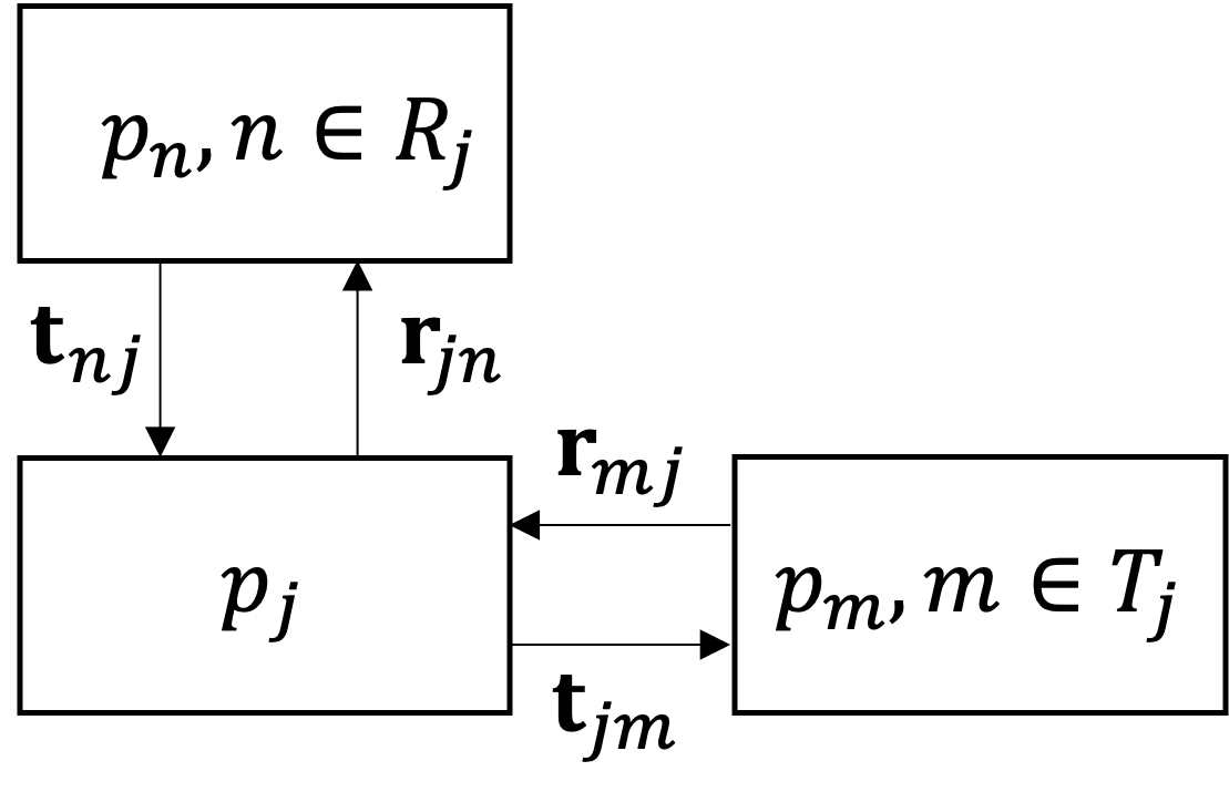
Fig. 5 Nonhierarchical target and response flow between subproblem \(j\) and its neighbors
We have two sets of consistency constraints related to subproblem \(j\):
The NHATC subproblem formulation is
ADMM coordinator
Now we explain how the ADMM algorithm works and how it penalizes violated inconsistency open constraints.
Defining inconsistencies
The scaled inconsistencies between each pair of linked variables are concatenated in the vector \({\bf q} \in {\bf R}^{n_{q}}\).
We use both \({\bf L}\) and \({\bf J}\) attributes to build the linking map \({\bf N}_{j} = [\bar{{\bf I}}_{j}, \underline{{\bf I}}_{j}]\) among variables of the MDO problem. In DMDO, the function responsible on building the linker matrix called set_pair which is one of the SubProblem class methods. Algorithm 1 shows how the linker matrix is built in DMDO.
             \begin{algorithm}
 \caption{Linker matrix}
 \begin{algorithmic}
 \STATE{Given ${\bf L}_{j}$, ${\bf D}_{j}$, ${\bf C}_{j}$, ${\bf N}_{j}$, $i$}
 \PROCEDURE{Build-linker-matrix}{}
     \STATE{$\bar{\bf l}_{j}=\{\}$ and $\underline{\bf l}_{j}=\{\}$}
     \FOR{$k \gets 1$ \textbf{to} $n_{\bf x}$}
       \IF{${\bf D}_{j}[k] = i \land  {\bf C}_{j}[k] \neq 0 \land {\bf L}_{j}[k] \notin \bar{\bf l}_{j}$}
         \STATE{$\bar{\bf l}_{j}[k] = {\bf D}_{j}[k]$}
         \FOR{$r \gets 1$ \textbf{to} $n_{\bf x}$}
           \IF{${\bf D}_{j}[r] \neq i \land {\bf L}_{j}[r] \notin \underline{\bf l}_{j} \land {\bf N}_{j}[i] = {\bf N}_{j}[r]$}
             \STATE{$\underline{\bf l}_{j}[r] = {\bf L}_{j}[r]$}
           \ENDIF
         \ENDFOR
       \ENDIF
     \ENDFOR
 \ENDPROCEDURE
 \end{algorithmic}
 \end{algorithm}
We also need to build a scaling vector \(\mathbf{s} \in \mathbb{R}^{n_{x}}_{+} \forall i \in \{1...n_{x}\}\) where
If one of the variables is not bounded, then scaling cannot be applied. Now we can define the inconsistency vector
\(\mathbf{q} \in \mathbb{R}^{n_{q}}\). Now, we need to define the single penalty function [16]
The penalty parameters \(\mathbf{v}_{t} \in \mathbb{R}^{n_{q}}\) and \(\mathbf{w}_{t} \in \mathbb{R}^{n_{q}}\) are initialized as
These parameters are updated at the end of the coordination loop using the method of multipliers scheme
where \(\beta > 1\) and \(0 \leq \gamma \leq 1\) are fixed parameters for the entire ADMM coordinator.
The coordinator is constructed as shown in the following code block.
NHATC main algorithm
In this section we will demonstrate how each step of the NHATC algorithm, shown in Algorithm 2, works and how it is implemented in DMDO.
             \begin{algorithm}
 \caption{NHATC}
 \begin{algorithmic}
 \STATE{Given $f : \mathbb{R}^{n} \mapsto  \mathbb{R} \cup \{ \infty \}$, variables declaration, initial values for the ADMM penalties, a starting point $x^{0} \in \Omega$ and extreme barrier function $f_{\Omega}(x)$}
 \PROCEDURE{MDO-Setup}{}
     \STATE{Group the variables in a single vector ${\bf x}$ where each variable is an instantiation of a data class that holds defined variables attributes}
     \STATE{Calculate the scaling vector ${\bf S}$}
     \STATE{Calculate the pairing/linking matrix using Algorithm 1.}
     \STATE{Define the disciplinary analyses $[{\bf y}_{j}] \leftarrow A_{j}({\bf x}[{\bf D}_{j}])$.}
     \STATE{Define the multidisciplinary analysis workflows included in each subproblem $[\mathbf{Y}_{j}] \leftarrow p_{\text{MDA}_{j}}(\mathbf{y}_{j}, \mathbf{x}[\mathbf{D}_{j}])$.}
     \STATE{Define subproblems $[f_{j}, \mathbf{g}_{j}, \mathbf{h}_{j}, y_{c_{j}}] \leftarrow p_{j}(\mathbf{Y}_{j}, \mathbf{x}[\mathbf{D}_{j}])$.}
     \STATE{Define the MDO problem.}
 \ENDPROCEDURE
 \PROCEDURE{Update}{}
     \STATE{Update the ADMM penalty parameters ${\bf w}$ and ${\bf v}$ based on the selected update scheme.}
 \ENDPROCEDURE
 \PROCEDURE{Inner-loop}{}
     \FOR{$j\leq n_{\text{subproblems}}$}
         \STATE{Get the linker matrix for the subproblem $p_{j}$}
         \STATE{Get the target variables ${\bf t}_{jm}$ for the subproblem $p_{j}$}
         \STATE{Prepare the design vector for $p_{j}$ based on ${\bf t}_{jm}, {\bf r}_{jn}, {\bf x}_{j}$  for the subproblem $p_{j}$}
         \STATE{Set the solver input parameters and options based on the optimization method selected}
         \STATE{Solve $p_{j}$ where open inconsistency constraints are calculated and penalized within the evaluator callable under the subproblem class}
     \ENDFOR
 \ENDPROCEDURE
 \PROCEDURE{Coordination-loop}{}
     \WHILE{\TRUE}
           \STATE{${\bf x}_{i} \gets {\bf x}_{i+1}$}
           \STATE{Go to Inner-loop()}
           \STATE{Update the design point with the best solution found from the inner loop ${\bf x}_{i+1} \gets {\bf x}^{*}$}
           \STATE{Calculate global inconsistency vector ${\bf q} = ({\bf x}_{i}-{\bf x}_{i+1}) \oslash {\bf S}$}
           \STATE{Go to Update()}
           \STATE{Go to Terminate()}
     \ENDWHILE
 \ENDPROCEDURE
 \PROCEDURE{Terminate}{}
     \IF{$\text{max}({\bf q}({\bf x})) \geq \epsilon_{stop} \lor i \leq n_{\text{budget}}$}
         \STATE $i \gets i+1$
     \ELSE
         \STATE stop
     \ENDIF
 \ENDPROCEDURE
 \end{algorithmic}
 \end{algorithm}
We will use a simple problem to demonstrate how the algorithm and its implementation work. The problem :math::mathcal{P} is defined as
The problem workflow is shown in Fig. 6 while its partitioned flow is depicted in Fig. 7.
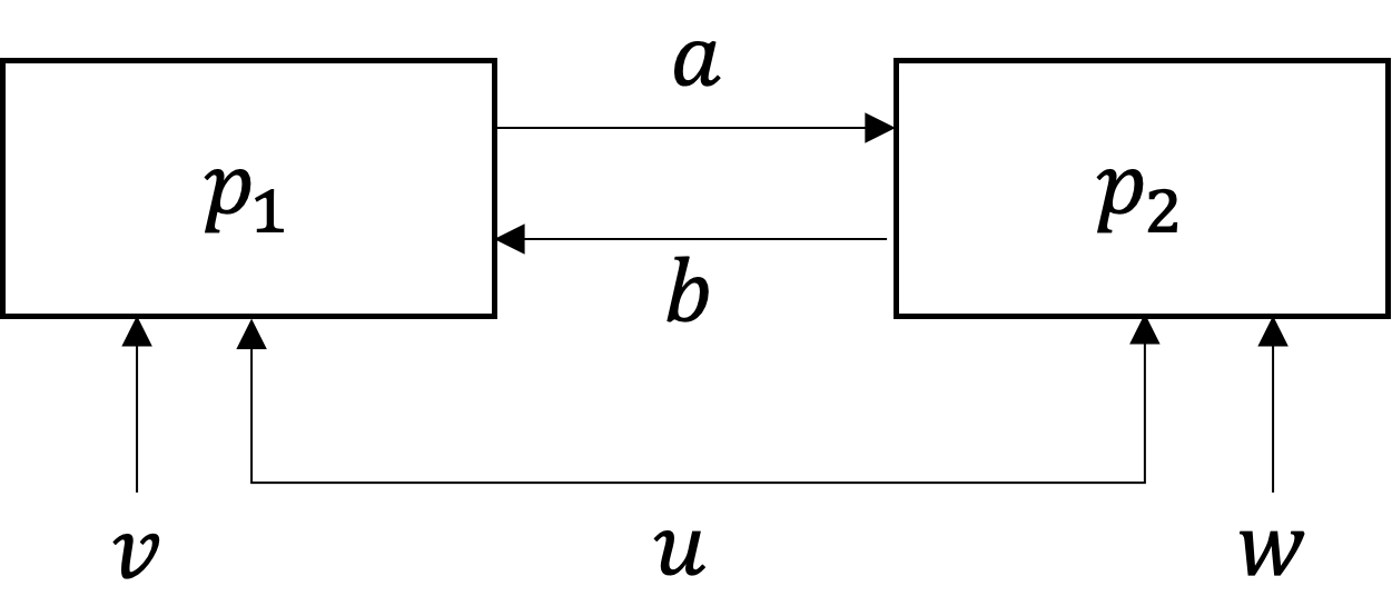
Fig. 6 Simple MDO workflow.
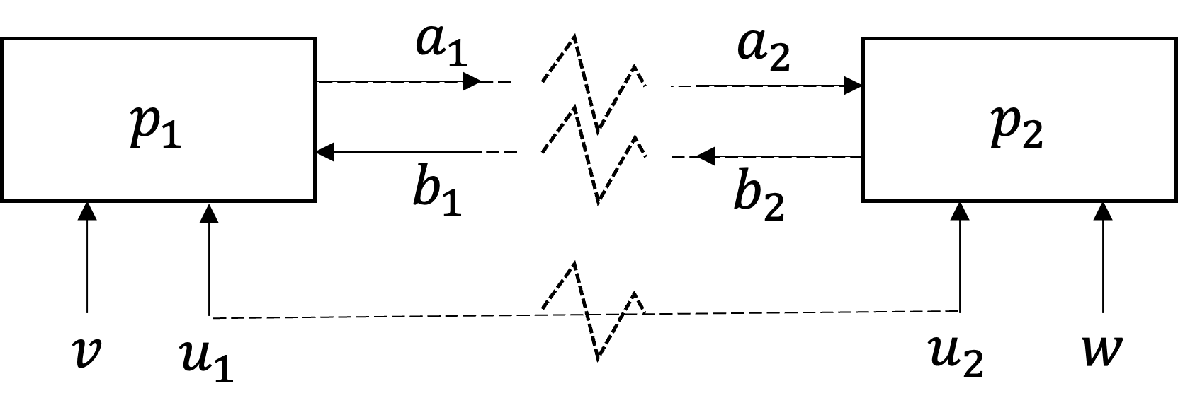
Fig. 7 Partitioned simple MDO problem.
The definition of subproblem 1 is
and subproblem 2 is
MDO setup
In this step, we either define the MDO problem setup manually or we introduce a serialized definition from a YAML input file to DMDO to autobuild the problem. We will start with the manual setup and then will show a sample of the YAML input file.
Variable declaration
The MDO workflow shown in Fig. 7 dictates that we have eight variables (after problem decomposition); two local variables \(w, v\) and six copies of coupling and shared variables \(u_{1}, u_{2}, a_{1}, a_{2}, b_{1}, b_{2}.\) So we start by regrouping those variables into a single variables vector
For each variable of \({\bf x}\), we declare the following list of attributes:
\(i\): Variable’s index where \(i \in \{0,1, ...,n_{x} \}\)
\(\mathbf{J}\): List of subproblem indices; this list holds the index of the subproblem where the variable \(x_{i}\) appears in.
\(\mathbf{N}\): List of variable names (In DMDO, we don’t assign the subproblem index to the variable name, so we introduce the variables copy by explicitly duplicating the name)
\(n_{v}\): List of each variable’s dimensions
\(\mathbf{C}_{t}\): List of coupling types; it holds the coupling type w.r.t to the subproblem index (not w.r.t the linked one) * Shared * Uncoupled * Feedforward * Feedback * Dummy
\(\mathbf{L}\): List of subproblem links; the index of the subproblem that the variable is linked to; each variable can be assigned to a scalar integer value for a single link or a list of integer values for multiple links
\(\mathbf{x}_{0}\): The initial design point
\(\mathbf{S}\): List of scaling factors
\(\bar{\mathbf{x}}\): Variable’s lower bound
\(\underline{\mathbf{x}}\): Variable’s upper bound
Without loss of generality, it is recommended to define scalar variables; however in DMDO, variables can be vectors of any length.
Let’s see how we can declare variables attributes in DMDO:
#  Variables setup
x = {}
X: List[variableData] = []
# Define variable names
N = ["u", "v", "a", "b", "u", "w", "a", "b"]
nx: int = len(N)
# Subproblem indices: Indices should be non-zero
J = [1,1,1,1,2,2,2,2]
# Subproblems links
L = [2, None, 2, 2, 1, None, 1, 1]
# Coupling types
Ct = [COUPLING_TYPE.SHARED, COUPLING_TYPE.UNCOUPLED, COUPLING_TYPE.FEEDFORWARD,
COUPLING_TYPE.FEEDBACK, COUPLING_TYPE.SHARED, COUPLING_TYPE.UNCOUPLED,
COUPLING_TYPE.FEEDBACK, COUPLING_TYPE.FEEDFORWARD]
# Lower bounds
lb = [0.]*8
# Upper bounds
ub = [10.]*8
# Baseline
x0 = [1.]*8
# Scaling
scaling = np.subtract(ub,lb)

# Inconsistency scaling
Qscaling=[]
# Create a dictionary for each variable
for i in range(nx):
  x[f"var{i+1}"] = {"index": i+1,
  "sp_index": J[i],
  f"name": N[i],
  "dim": 1,
  "value": 0.,
  "coupling_type": Ct[i],
  "link": L[i],
  "baseline": x0[i],
  "scaling": scaling[i],
  "lb": lb[i],
  "value": x0[i],
  "ub": ub[i]}
  Qscaling.append(1/scaling[i] if 1/scaling[i] != np.inf and 1/scaling[i] != np.nan else 1.)


# Instantiate the variableData class for each variable using its according dictionary
for i in range(nx):
  X.append(variableData(**x[f"var{i+1}"]))
Disciplinary analyses
After constructing the list of the variablesData class instantiations, then we can instantiate the process class of each disciplinary analysis (DA). For the sake of simplicity, we use callable functions to execute the analysis.
def A1(x):
  LAMBDA = 0.0
  for i in range(len(x)):
    if x[i] == 0.:
      x[i] = 1e-12
  return math.log(x[0]+LAMBDA) + math.log(x[1]+LAMBDA) + math.log(x[2]+LAMBDA)

def A2(x):
  LAMBDA = 0.0
  for i in range(len(x)):
    if x[i] == 0.:
      x[i] = 1e-12
  return np.divide(1., (x[0]+LAMBDA)) + np.divide(1., (x[1]+LAMBDA)) + np.divide(1., (x[2]+LAMBDA))
We introduce the variableData along with the analysis callable functions to the DA process class instantiations:
# Analyses setup; construct disciplinary analyses
DA1: process = DA(inputs=[X[0], X[1], X[3]],
outputs=[X[2]],
blackbox=A1,
links=2,
coupling_type=COUPLING_TYPE.FEEDFORWARD
)

DA2: process = DA(inputs=[X[4], X[5], X[6]],
outputs=[X[7]],
blackbox=A2,
links=1,
coupling_type=COUPLING_TYPE.FEEDFORWARD
)
Multidisciplinary analysis
The response outputs of \(A_{j}(\mathbf{x}[\mathbf{D}_{j}])\) will be used to evaluate the MDA processes of each MDO subproblem.
# MDA setup; construct subproblems MDA
sp1_MDA: process = MDA(nAnalyses=1, analyses = [DA1], variables=[X[0], X[1], X[3]], responses=[X[2]])
sp2_MDA: process = MDA(nAnalyses=1, analyses = [DA2], variables=[X[4], X[5], X[6]], responses=[X[7]])
The vector \(\mathbf{Y}_{j}\) should include all the dependent design variables including the coupling variables of the subproblem \(j\) in the same order of the MDA process returned outputs.
ADMM coordinator
The coordinator object is constructed as shown in the following code block:
 # Construct the coordinator
coord = ADMM(beta = 1.3,
nsp=2,
budget = 50,
index_of_master_SP=1,
display = True,
scaling = Qscaling,
mode = "serial",
M_update_scheme= w_scheme.MEDIAN,
store_q_io=True
)
Subproblem j
Now we can formulate the optimization subproblem \(j\) at iteration \(i\) as follows
The following code block shows how to construct the MDO subproblems
def opt1(x, y):
  return [sum(x)+y[0], [0.]]

def opt2(x, y):
  return [0., [x[1]+y[0]-10.]]

# Construct subproblems
# Construct subproblems
sp1 = SubProblem(nv = 3,
index = 1,
vars = [X[0], X[1], X[3]],
resps = [X[2]],
is_main=1,
analysis= sp1_MDA,
coordination=coord,
opt=opt1,
fmin_nop=np.inf,
budget=20,
display=False,
psize = 1.,
pupdate=PSIZE_UPDATE.LAST,
freal=2.625)

sp2 = SubProblem(nv = 3,
index = 2,
vars = [X[4], X[5], X[6]],
resps = [X[7]],
is_main=0,
analysis= sp2_MDA,
coordination=coord,
opt=opt2,
fmin_nop=np.inf,
budget=20,
display=False,
psize = 1.,
pupdate=PSIZE_UPDATE.LAST
)
MDO
Finally, we construct the MDAO process as follows:
# Construct MDO workflow
MDAO: MDO = MDO(
Architecture = MDO_ARCHITECTURE.IDF,
Coordinator = coord,
subProblems = [sp1, sp2],
variables = X,
responses = [X[2], X[7]],
fmin = np.inf,
hmin = np.inf,
display = False,
inc_stop = 1E-9,
stop = "Iteration budget exhausted",
tab_inc = [],
noprogress_stop = 100
)

coord2 = copy.deepcopy(coord)
coord2.budget = 100
sp_12 = copy.deepcopy(sp1)
sp_12.budget = 10
sp_12.coord = coord2
sp_22 = copy.deepcopy(sp2)
sp_22.coord = coord2

sp_22.budget = 10
MDAO2 = copy.deepcopy(MDAO)
MDAO2.subProblems = [sp_12, sp_22]
MDAO2.Coordinator = coord2
MDAO2.display = True
MDAO2.run()
# Run the MDO problem
out = MDAO.run()
Results display
0 || qmax: 9.57399606704712e-08 || Obj: 1.9999990426003933 || dx: 1.7320508075691419 || max(w): 1.0
Highest inconsistency : u_2 to u_1
1 || qmax: 9.765662252902985e-05 || Obj: 1.9990234337747097 || dx: 1.7320510828730173 || max(w): 1.6900000000000002
Highest inconsistency : u_2 to u_1
2 || qmax: 0.1 || Obj: 1.0 || dx: 2.0 || max(w): 2.8561000000000005
Highest inconsistency : u_2 to u_1
3 || qmax: 0.1 || Obj: 1.0 || dx: 2.0 || max(w): 4.826809000000002
Highest inconsistency : u_2 to u_1
4 || qmax: 0.050097656250000004 || Obj: 1.4990234375 || dx: 1.803046731555873 || max(w): 8.157307210000004
Highest inconsistency : u_2 to u_1
5 || qmax: 0.012402343750000001 || Obj: 2.1240234375 || dx: 1.7364854773505354 || max(w): 13.785849184900009
Highest inconsistency : b_2 to b_1
6 || qmax: 0.0016601562500000002 || Obj: 1.9833984375 || dx: 1.732130368037418 || max(w): 23.298085122481016
Highest inconsistency : u_2 to u_1
7 || qmax: 0.0 || Obj: 2.0 || dx: 1.7320508075688772 || max(w): 39.37376385699292
Highest inconsistency : u_2 to u_1
Stop: qmax = 0.0 < 1e-09
Stop: qmax = 4.656612873077393e-10 < 1e-09
Multipliers update
def update_multipliers(self):
  self.v = np.add(self.v, np.multiply(
          np.multiply(np.multiply(2, self.w), self.w), self.q))
  self.calc_inconsistency_old()
  self.q_stall = np.greater(np.abs(self.q), self.gamma*np.abs(self.qold))
  increase_w = []
  if self.M_update_scheme == w_scheme.MEDIAN:
    for i in range(self.q_stall.shape[0]):
      increase_w.append(2. * ((self.q_stall[i]) and (np.greater_equal(np.abs(self.q[i]), np.median(np.abs(self.q))))))
  elif self.M_update_scheme == w_scheme.MAX:
    tc = np.greater_equal(np.abs(self.q), np.max(np.abs(self.q)))
    for i in range(self.q_stall.shape[0]):
      increase_w.append(self.q.shape[0] * (self.q_stall[i] and tc[i]))
  elif self.M_update_scheme == w_scheme.NORMAL:
    increase_w = self.q_stall
  elif self.M_update_scheme == w_scheme.RANK:
    temp = self.q.argsort()
    rank = np.empty_like(temp)
    rank[temp] = np.arange(len(self.q))
    increase_w = np.multiply(np.multiply(2, self.q_stall), np.divide(rank, np.max(rank)))
  else:
    raise Exception(IOError, "Multipliers update scheme is not recognized!")

  for i in range(len(self.w)):
    self.w[i] = copy.deepcopy(np.multiply(self.w[i], np.power(self.beta, increase_w[i])))

  self.w
Inner loop
""" ADMM inner loop """
for s in range(len(self.subProblems)):
  if iter == 0:
    self.subProblems[s].coord = copy.deepcopy(self.Coordinator)
    self.subProblems[s].set_pair()
    self.xavg = self.subProblems[s].coord._linker
    self.Coordinator.v = [0.] * len(self.subProblems[s].coord._linker[0])
    self.Coordinator.w = [1.] * len(self.subProblems[s].coord._linker[0])
  else:
    self.subProblems[s].coord.master_vars = copy.deepcopy(self.Coordinator.master_vars)

  out_sp = self.subProblems[s].solve(self.Coordinator.v, self.Coordinator.w)
  self.Coordinator = copy.deepcopy(self.subProblems[s].coord)
  if self.subProblems[s].index == self.Coordinator.index_of_master_SP:
    self.fmin = self.subProblems[s].fmin_nop
    if self.subProblems[s].solver == "OMADS":
      self.hmin = out_sp["hmin"]
    else:
      self.hmin = [0.]
Coordination-loop
def run(self):
  global eps_fio, eps_qio
  # Note: once you run MDAO, the data stored in eps_fio and eps_qio shall be deleted. It is recommended to store such data to a different variable before running another MDAO
  eps_fio = []
  eps_qio = []
  """ Run the MDO process """
  #  COMPLETE: fix the setup of the local (associated with SP) and global (associated with MDO) coordinators
  for iter in range(self.Coordinator.budget):
    if iter > 0:
      self.Coordinator.master_vars_old = copy.deepcopy(self.Coordinator.master_vars)
    else:
      self.Coordinator.master_vars_old = copy.deepcopy(self.variables)
      self.Coordinator.master_vars = copy.deepcopy(self.variables)

    """ ADMM inner loop """
    for s in range(len(self.subProblems)):
      if iter == 0:
        self.subProblems[s].coord = copy.deepcopy(self.Coordinator)
        self.subProblems[s].set_pair()
        self.xavg = self.subProblems[s].coord._linker
        self.Coordinator.v = [0.] * len(self.subProblems[s].coord._linker[0])
        self.Coordinator.w = [1.] * len(self.subProblems[s].coord._linker[0])
      else:
        self.subProblems[s].coord.master_vars = copy.deepcopy(self.Coordinator.master_vars)

      out_sp = self.subProblems[s].solve(self.Coordinator.v, self.Coordinator.w)
      self.Coordinator = copy.deepcopy(self.subProblems[s].coord)
      if self.subProblems[s].index == self.Coordinator.index_of_master_SP:
        self.fmin = self.subProblems[s].fmin_nop
        if self.subProblems[s].solver == "OMADS":
          self.hmin = out_sp["hmin"]
        else:
          self.hmin = [0.]

    """ Display convergence """
    dx = self.get_master_vars_difference()
    if self.display:
      print(f'{iter} || qmax: {np.max(np.abs(self.Coordinator.q))} || Obj: {self.fmin} || dx: {dx} || max(w): {np.max(self.Coordinator.w)}')
      index = np.argmax(self.Coordinator.q)
      print(f'Highest inconsistency : {self.Coordinator.master_vars[self.Coordinator._linker[0,index]-1].name}_'
        f'{self.Coordinator.master_vars[self.Coordinator._linker[0,index]-1].link} to '
          f'{self.Coordinator.master_vars[self.Coordinator._linker[1,index]-1].name}_'
        f'{self.Coordinator.master_vars[self.Coordinator._linker[1,index]-1].link}')
    """ Update LM and PM """
    self.Coordinator.update_multipliers()

    """ Stopping criteria """
    self.tab_inc.append(np.max(np.abs(self.Coordinator.q)))
    stop: bool = self.check_termination_critt(iter)

    if stop:
      break
    self.eps_qio = copy.deepcopy(eps_qio)
    self.eps_fio = copy.deepcopy(eps_fio)
  return self.Coordinator.q