Benchmark Results And Discussion

This page reports the benchmark described in Benchmark Problems And Setup: 4080 fits of four surrogate models on 51 outputs of seven engineering problems, with 5 random training samples at each of 4 training-set sizes. All numbers are medians over seeds on the fixed test split unless stated otherwise. Every figure is generated from BM/results/raw_results.csv by BM/make_doc_figures.py.

Key findings

Summary

1. A few hundred samples are enough for most outputs. With 400 samples, Kriging and the ensemble meet all three acceptance criteria on 33 of 51 outputs. Leaving out the 14-input truss and the three non-smooth outputs, they pass 30 of the remaining 33. Three of the seven problems are passed in full by at least one model (Fig. 1).

2. Accuracy comes early. Kriging already passes 19 outputs with 50 samples and 31 with 200. Beyond 200 samples the gains are small (Fig. 4).

3. The ensemble is a safe default. At \(n = 400\) it is within 0.02 \(R^2\) of the best of its three experts on 88% of outputs, and it beats the worst expert on every output from \(n = 100\) upwards, without knowing in advance which expert is best (Fig. 6).

4. Results are stable. The median seed-to-seed standard deviation of test \(R^2\) falls from about 0.05 at \(n = 50\) to 0.003 at \(n = 400\) for Kriging and the ensemble (Fig. 7).

5. Cost and accuracy trade off in a predictable way. LS and RBF fit in milliseconds and pass 20 and 27 outputs. Kriging and the ensemble pass 33 but cost seconds to minutes per output at \(n = 400\) (Fig. 5).

6. The failures are informative, not random. They concentrate on three deliberately non-smooth outputs, on the heavy-tailed member stresses of the 14-input truss, and on quadratic LS for strongly non-polynomial responses. Almost every failure is a tail failure (\(R^2\) and worst-case error) rather than a large typical error.

Overall pass rates

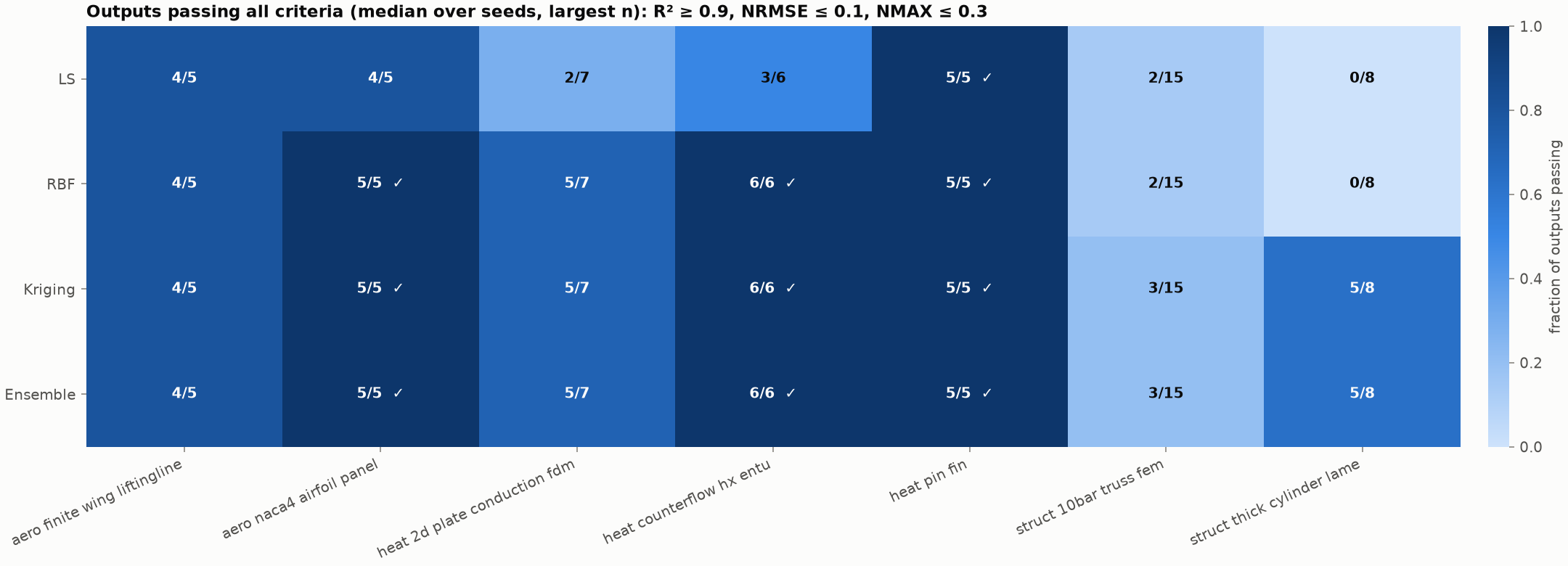
Fig. 1 Outputs passing all three criteria at \(n = 400\) (median over 5 seeds), per model and dataset. A tick marks a dataset passed in full.

Fig. 1 summarizes the verdict. The pin fin is passed in full by all four models, and the heat exchanger and the airfoil by every model except the quadratic LS.

Model	Outputs passing (of 51)	Datasets passed in full (of 7)	Mean rank by test \(R^2\)
Kriging	33	3	1.43
Ensemble	33	3	1.71
RBF	27	3	3.12
LS	20	1	3.75

Kriging has the highest median \(R^2\) on 34 outputs, the ensemble on 15 and LS on 2. Fig. 2 resolves this output by output. Every output is fitted to \(R^2 > 0.9\) by at least one model, except the three non-smooth location outputs, three cylinder stress outputs (≈ 0.87) and most truss displacement and stress outputs.

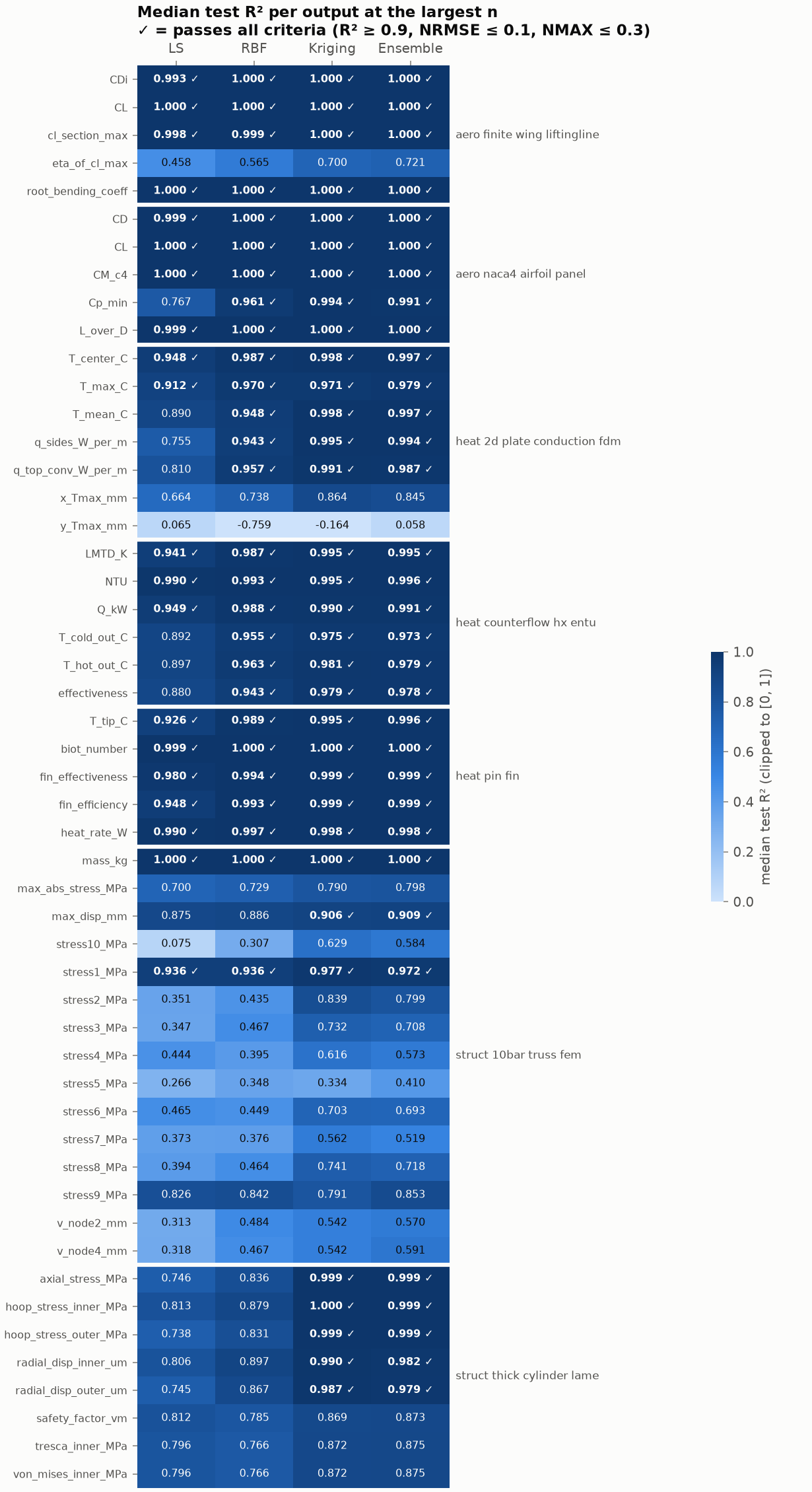
Fig. 2 Median test \(R^2\) for all 51 outputs at \(n = 400\), grouped by dataset. Bold cells with a tick pass all three criteria. Values below 0 are shown at the lightest color.

Learning curves

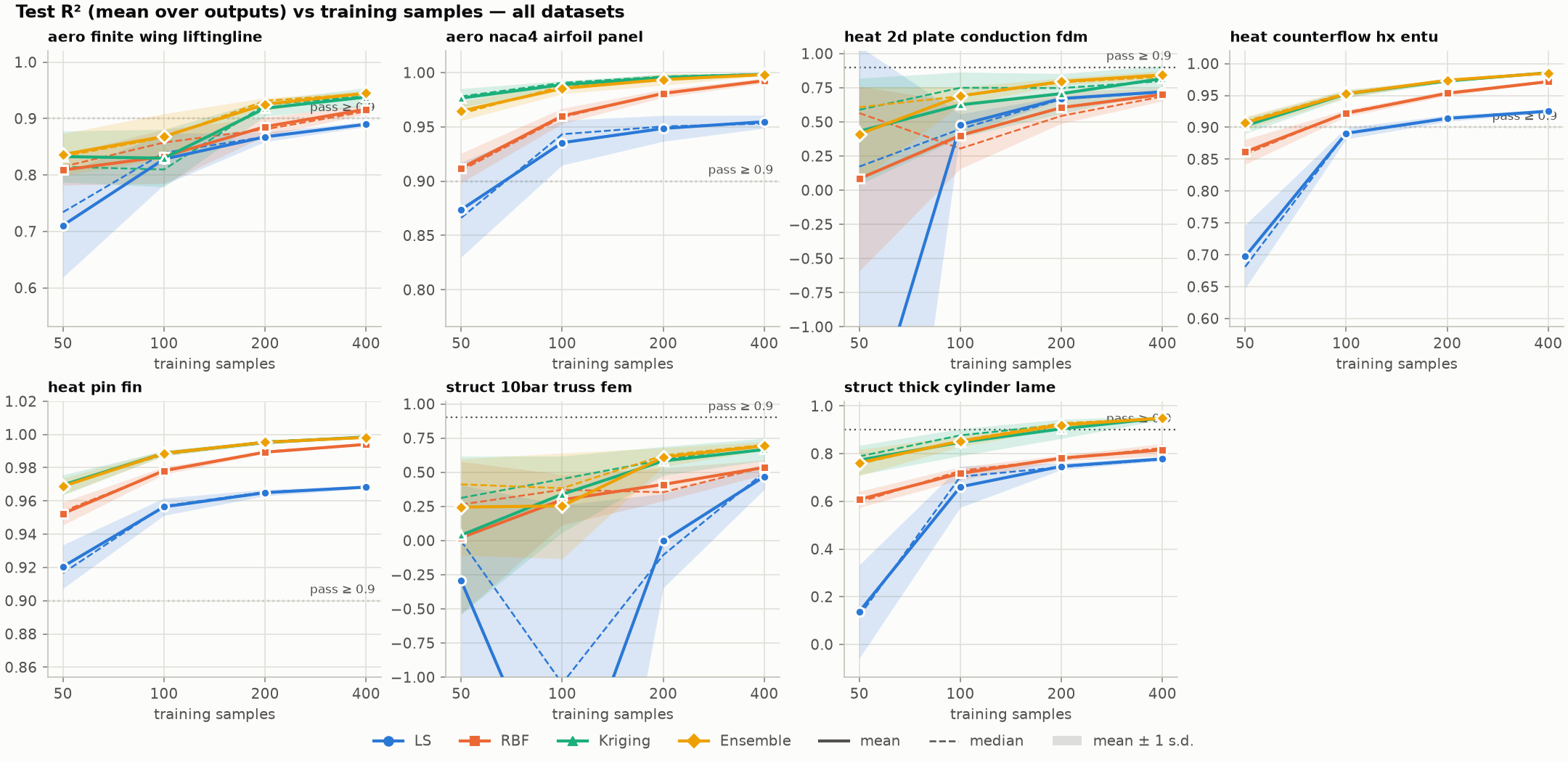
Fig. 3 Test \(R^2\) averaged over each dataset’s outputs against the number of training samples. The solid line is the mean over seeds, the dashed line the median, and the band ±1 standard deviation.

Every model improves monotonically with more data on every dataset, apart from seed noise at \(n \le 100\) (Fig. 3). The dataset-averaged median \(R^2\) at \(n = 400\) is:

Dataset	LS	RBF	Kriging	Ensemble
aero_naca4_airfoil_panel	0.953	0.992	0.999	0.998
heat_pin_fin	0.968	0.994	0.998	0.998
heat_counterflow_hx_entu	0.925	0.971	0.986	0.986
struct_thick_cylinder_lame	0.775	0.824	0.948	0.948
aero_finite_wing_liftingline	0.890	0.913	0.940	0.944
heat_2d_plate_conduction_fdm	0.718	0.686	0.798	0.829
struct_10bar_truss_fem	0.499	0.538	0.701	0.701

Two features stand out. The quadratic LS saturates: its curves flatten well below the others on the cylinder, the heat exchanger and the plate, because a degree-2 polynomial can’t represent those responses whatever the sample size. The interpolating models (RBF and Kriging) keep improving. Second, the gap between the solid mean and dashed median lines at small \(n\) shows that the mean is pulled down by a few poor fits. The median, which the acceptance criteria use, is the more robust summary.

Sample efficiency

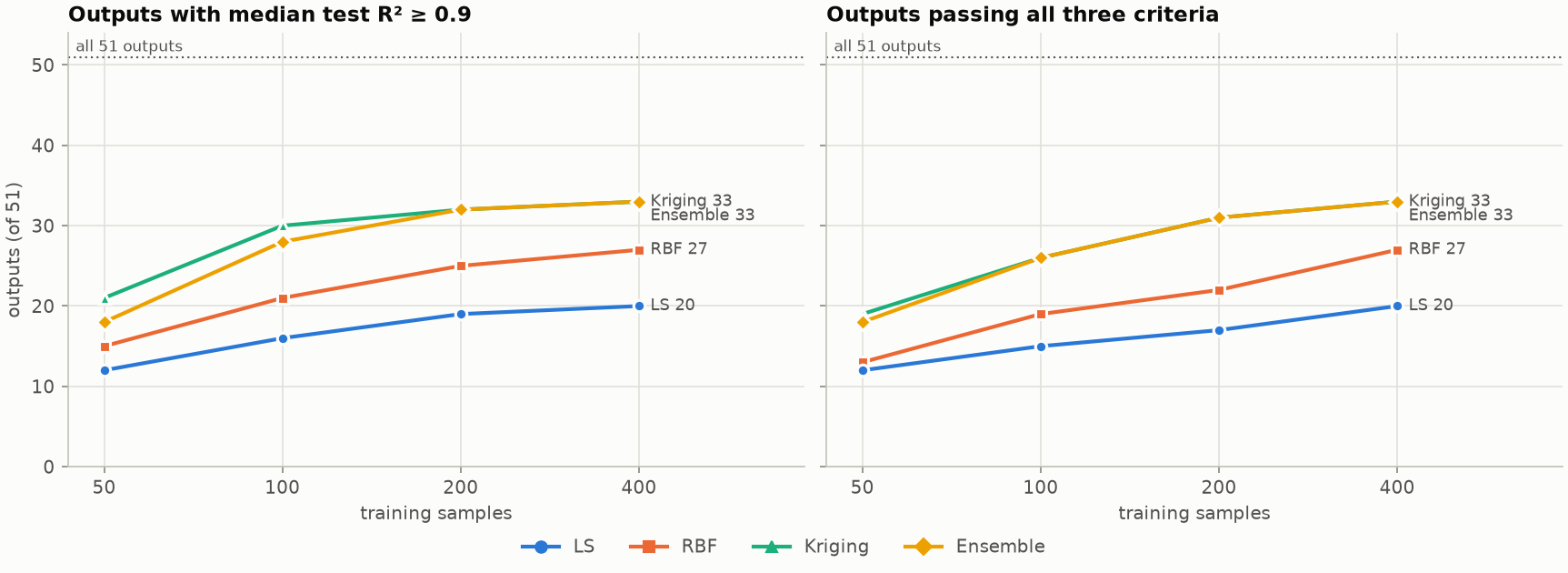
Fig. 4 Number of outputs (of 51) with median \(R^2 \ge 0.9\) (left) and passing all three criteria (right), as a function of training-set size.

Fig. 4 is the most direct evidence for the premise that surrogates can be built from few samples:

Training samples	50	100	200	400
Kriging (all criteria)	19	26	31	33
Ensemble (all criteria)	18	26	31	33
RBF (all criteria)	13	19	22	27
LS (all criteria)	12	15	17	20

Kriging reaches 94% of its final pass count (31 of 33) with 200 samples, and 58% with only 50. Doubling from 200 to 400 samples adds two outputs. For the problems in this suite, the useful budget is therefore in the low hundreds of evaluations, which is affordable even for simulations that take minutes to hours per run.

Accuracy versus training cost

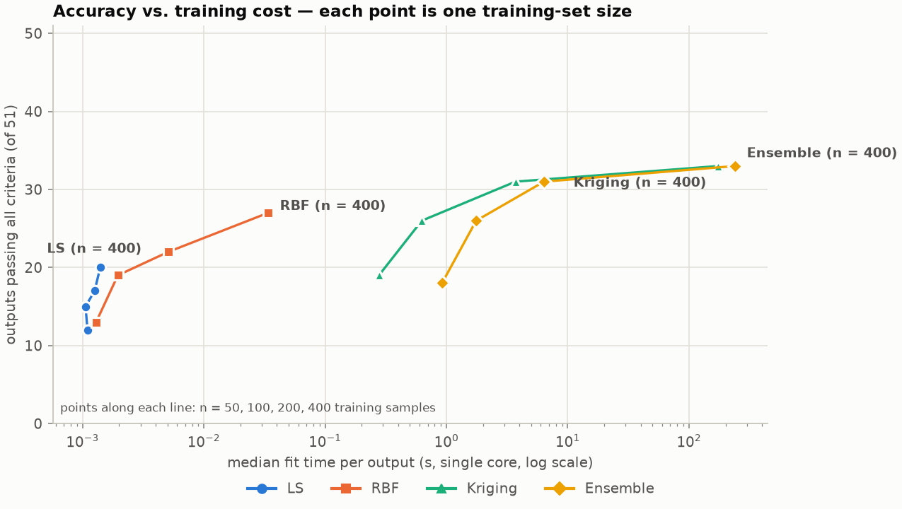
Fig. 5 Outputs passing all criteria against the median fit time per output. Each line follows one model through \(n = 50, 100, 200, 400\).

Fig. 5 shows the two regimes of the package. LS and RBF fit in 1–34 ms per output at \(n = 400\), cheap enough to refit inside an optimization loop at every iteration. Kriging and the ensemble buy the extra 6–13 outputs with fits of 0.3–0.9 s at \(n = 50\), 3.7–6.4 s at \(n = 200\) and 3–4 minutes at \(n = 400\).

Note

Fit times were measured while 24 fits ran concurrently, one BLAS thread each, so they are pessimistic for a single fit on an idle machine. The ranking and the orders of magnitude are what matter. The cost of Kriging is dominated by the likelihood optimization (Algorithm 4), whose gradient is currently estimated by finite differences.

The ensemble costs 1.4–3× as much as Kriging (more at small \(n\)), because the cross-validation used to set its weights refits all three experts. In return it removes the need to pick a model, as the next section shows.

The ensemble as a default

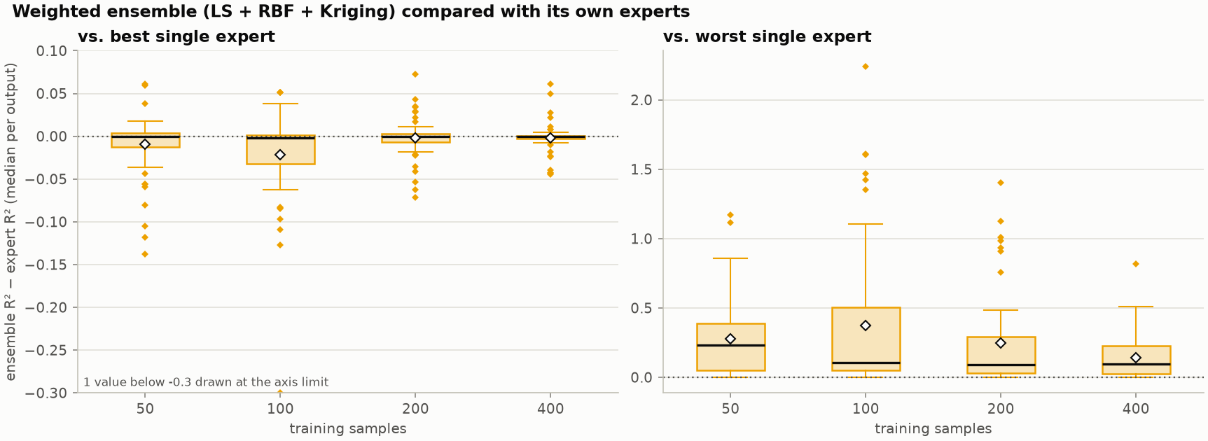
Fig. 6 Difference between the ensemble’s median test \(R^2\) and that of its best (left) and worst (right) single expert, one value per output. Boxes span the interquartile range; the black line is the median and the diamond the mean.

The weighted ensemble combines LS, RBF and Kriging with weights proportional to their inverse cross-validated MSE (Theory And Algorithms). Fig. 6 compares it with its own experts:

• Against the best expert (left) the median difference is essentially zero at every size (−0.0002 to −0.002). At \(n = 400\) the ensemble is within 0.02 \(R^2\) of the best expert on 88% of outputs and at least as good on 29%.

• Against the worst expert (right) it is better on 98% of outputs at \(n = 50\) and on 100% from \(n = 100\), with a median gain of about 0.1 \(R^2\).

Which single model is best varies by output: Kriging on most, LS on smooth near-polynomial outputs such as the truss mass. The ensemble tracks the best one automatically. When the user can’t afford to benchmark every model on their problem, the ensemble is the choice that is almost never much worse than the best.

Stability across training samples

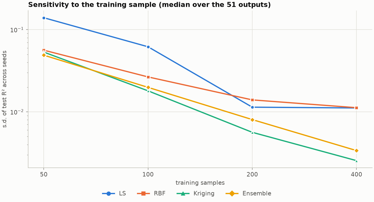
Fig. 7 Standard deviation of test \(R^2\) across the 5 random training samples, median over the 51 outputs.

An engineer builds a surrogate from one sample of their model, so the spread across seeds measures how much the result depends on that particular sample (Fig. 7). For Kriging, the median standard deviation of \(R^2\) falls from 0.053 at \(n = 50\) to 0.0025 at \(n = 400\) (21×), and for the ensemble from 0.049 to 0.0034. LS is the most sample-sensitive at small \(n\) (0.14 at \(n = 50\)), because a full quadratic (28 coefficients for \(d = 6\), 120 for the truss) fitted to 50 points is barely determined. Its variability then flattens at about 0.011, as do RBF’s: when a model is limited by its form rather than its data, more samples no longer reduce the spread.

Per-problem discussion

Smooth problems: pin fin, heat exchanger, airfoil

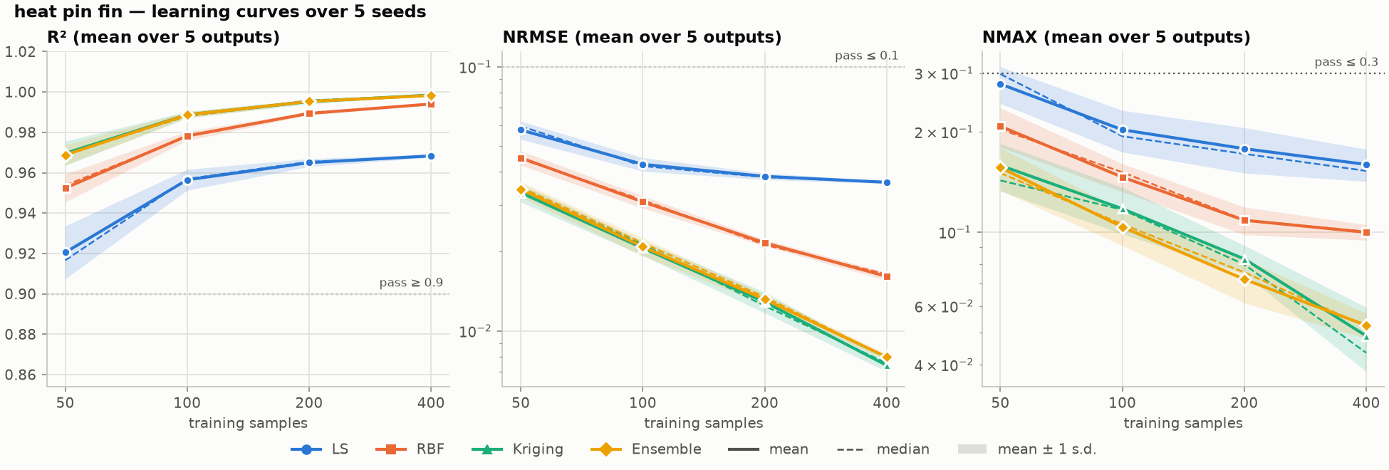
Fig. 8 Pin fin: learning curves of the three metrics, averaged over the 5 outputs.

On the pin fin every model passes every output (Fig. 8), and Kriging and the ensemble reach \(R^2 \approx 0.97\) with only 50 samples. On the heat exchanger and the airfoil, RBF, Kriging and the ensemble pass every output. LS misses three heat-exchanger outputs (the outlet temperatures and the effectiveness, \(R^2 \approx 0.88\)–0.90) and the airfoil’s \(C_{p,\min}\) (\(R^2 = 0.77\)). Those are the most non-polynomial responses: saturation of \(\varepsilon(\mathrm{NTU})\) and the suction-peak behaviour of \(C_{p,\min}\). These problems represent the typical case the package is designed for: smooth responses over a moderate number of inputs.

Cylinder: closed form, but rational

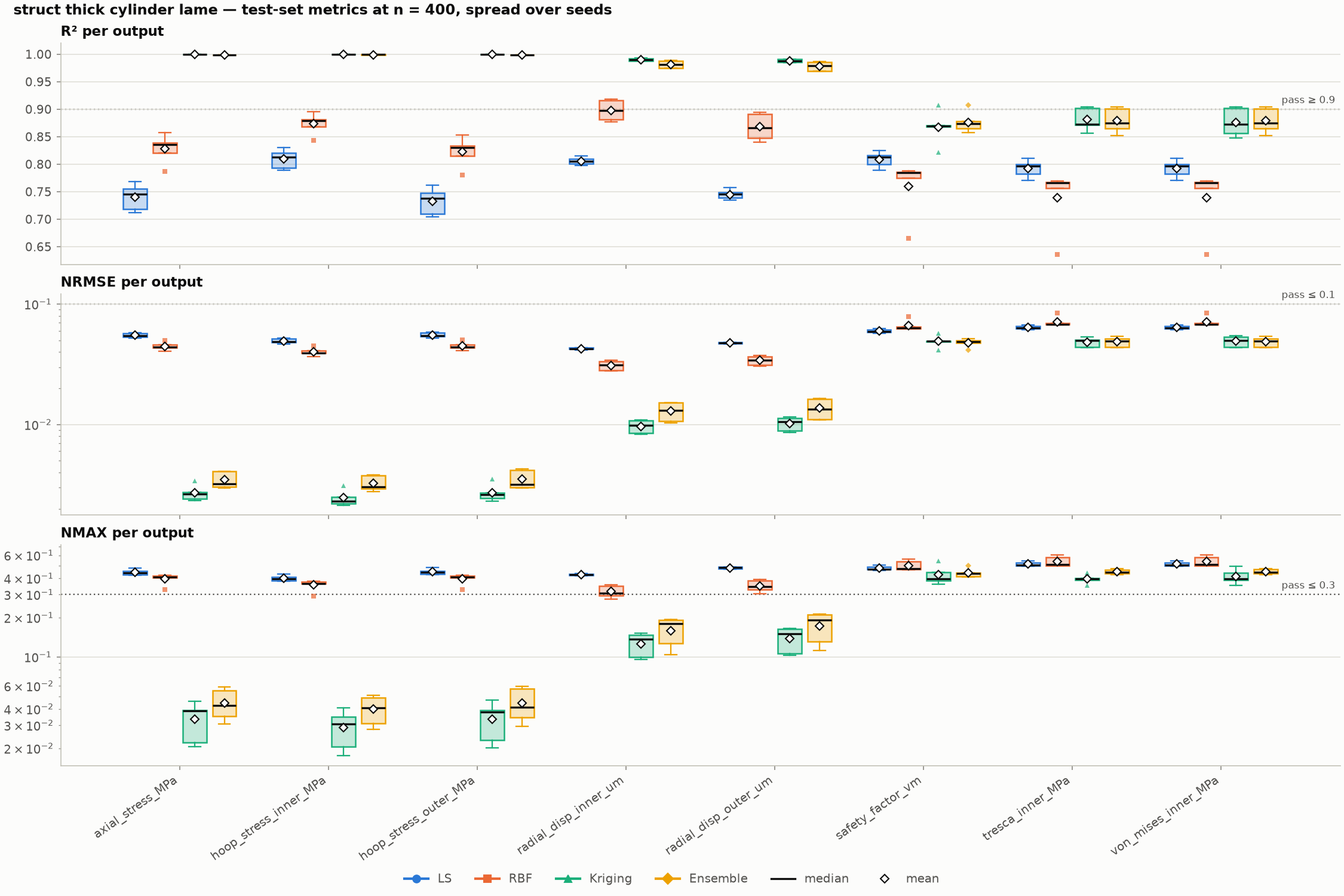
Fig. 9 Thick cylinder: spread over seeds of each metric per output at \(n = 400\).

The Lamé solution is exact and smooth, yet LS and RBF pass none of its 8 outputs (Fig. 9). The stresses are rational functions of the radii that are strongly curved near thin walls, which a quadratic can’t follow, and the cubic RBF needs more points to resolve them. Kriging fits the hoop, axial and displacement outputs to \(R^2 \ge 0.987\), and the ensemble to \(R^2 \ge 0.979\). The remaining three failures (von Mises, Tresca and safety factor, \(R^2 \approx 0.87\) in log space) all share the factor \(p_i - p_o\) that vanishes inside the sampled domain (see Benchmark Problems And Setup), and they also fail NMAX near that singularity. Von Mises and Tresca have identical scores because, at the bore, one is a constant multiple of the other.

Truss: the high-dimensional case

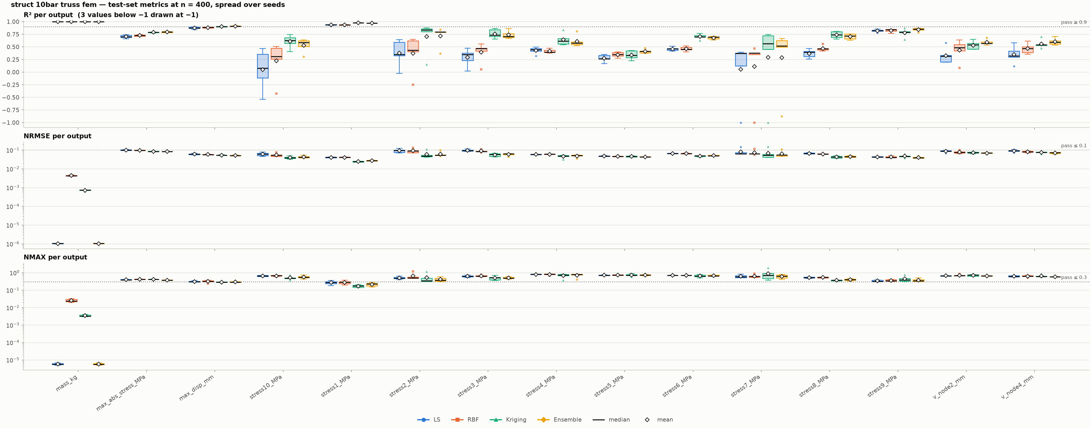
Fig. 10 10-bar truss: spread over seeds of each metric per output at \(n = 400\).

With 14 inputs, the truss is the problem where 400 samples are clearly not enough (Fig. 10). The mass, which is bilinear in density and areas, is fitted to \(R^2 = 1.000\) by every model, and the always-positive stress in member 1 to \(R^2 \ge 0.93\). The other member stresses and the nodal displacements behave like \(1/A_e\) in the loaded members, which produces heavy, signed tails that can’t be log-transformed. Their \(R^2\) is 0.33–0.84 for Kriging, while their NRMSE is only 4–8% of the range. The surrogate captures the bulk of the response but misses the extreme members. The learning curve in Fig. 3 is still rising at \(n = 400\): this problem needs more data, a transformation of the areas (for example fitting in terms of \(1/A_e\)), or dimension reduction with the collinearity filter.

Non-smooth outputs: wing and plate

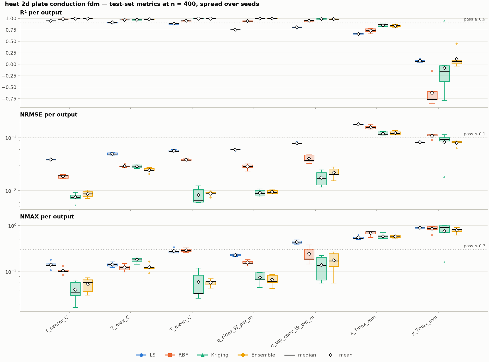
Fig. 11 Plate conduction: spread over seeds of each metric per output at \(n = 400\). The two location outputs are non-smooth by construction.

The location outputs \(x_{T_{\max}}\), \(y_{T_{\max}}\) and \(\eta_{c_{l,\max}}\) are piecewise constant, jumping between grid points, and no model passes them (\(R^2 \le 0.87\), and as low as −0.76 for \(y_{T_{\max}}\)). Fig. 11 shows that this doesn’t spill over to the other outputs of the same problems: the plate temperatures and heat flows pass for RBF, Kriging and the ensemble, and every other wing output passes for all four models. These outputs were included to confirm that the criteria do reject a surrogate when the target isn’t a continuous function of the inputs. They do.

Why outputs fail

Of the 204 (model, output) pairs, 91 fail. Every one of them fails the \(R^2\) threshold, 87 also fail the worst-case NMAX threshold, but only 11 fail NRMSE. The typical error is small almost everywhere. What fails is the explained variance and the worst case, both of which are driven by the tails of the response:

• Heavy or signed tails (truss stresses and displacements, cylinder equivalent stresses): a small number of extreme test points carry most of the variance.

• Discontinuities (the three location outputs): no smooth interpolant can reproduce a jump.

• Model form (LS): a global quadratic saturates on rational or exponential responses.

This is also the practical message for users. A good NRMSE combined with a poor \(R^2\) or NMAX points to tails or jumps in the data. The remedies are better input and output transformations or more samples in the extreme region, not a different interpolant.

Threats to validity

• Noise-free data. All datasets are deterministic, so the benchmark measures approximation error only. With noisy data, interpolating models (RBF, Kriging with a tiny nugget) need regularization. Adding 1–5% output noise, as the dataset README suggests, is a natural extension.

• Fixed, untuned configurations. One setting per model is used for all problems. Per-problem tuning (the LS degree, the RBF kernel, Kriging’s correlation exponent) would improve some results. The benchmark reflects out-of-the-box behaviour.

• Single-output fitting. Each of the 51 outputs has its own surrogate. Correlations between outputs of the same problem are not exploited.

• Fixed test split. Seeds vary the training sample and the model’s internal randomness, not the test set. The test sets are large (135–573 points), so test-sampling noise is small compared with the effects discussed here.

• Timing under load. Fit times were measured with 24 concurrent processes (see the note in the section on training cost above).

Conclusion

The benchmark supports the premise of ddmo with evidence rather than anecdote:

• Across seven engineering problems from three disciplines, a few hundred samples give surrogates that meet strict accuracy criteria on nearly all smooth outputs.

• Kriging is the most accurate and most sample-efficient family.

• RBF and LS are orders of magnitude cheaper to train and remain adequate for the smoother responses.

• The weighted ensemble matches the best family without the user having to know which one that is.

The failures are concentrated where theory predicts them (discontinuities, singular or heavy-tailed responses, and 14 inputs with only 400 samples), and the metrics make those cases visible instead of averaging them away.

Complete per-dataset figures

The learning curves and box plots for all seven datasets, in the same format as the figures above.

Learning curves

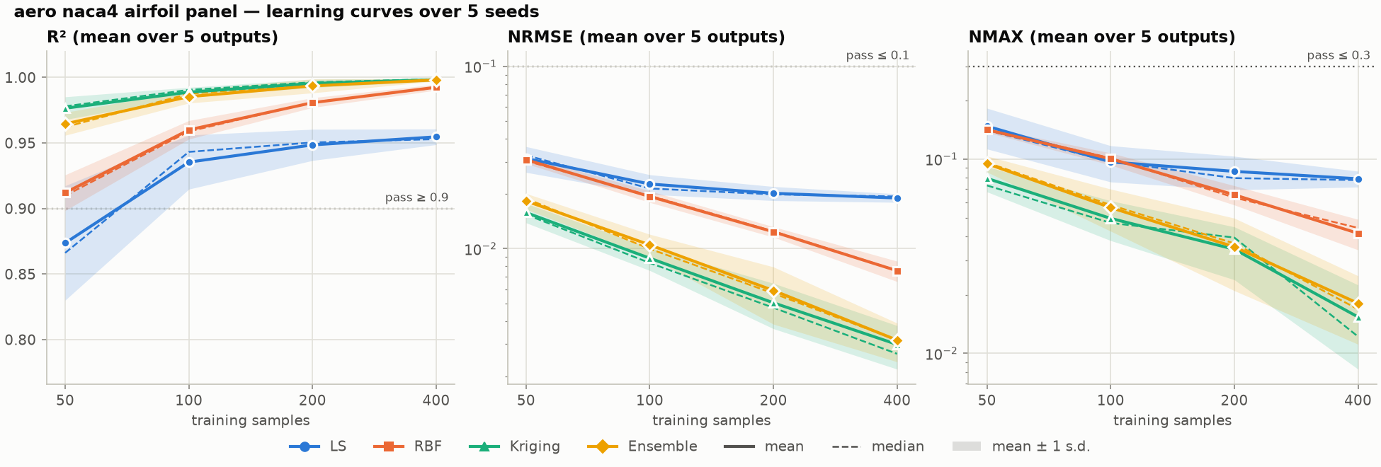
Fig. 12 Airfoil panel method.

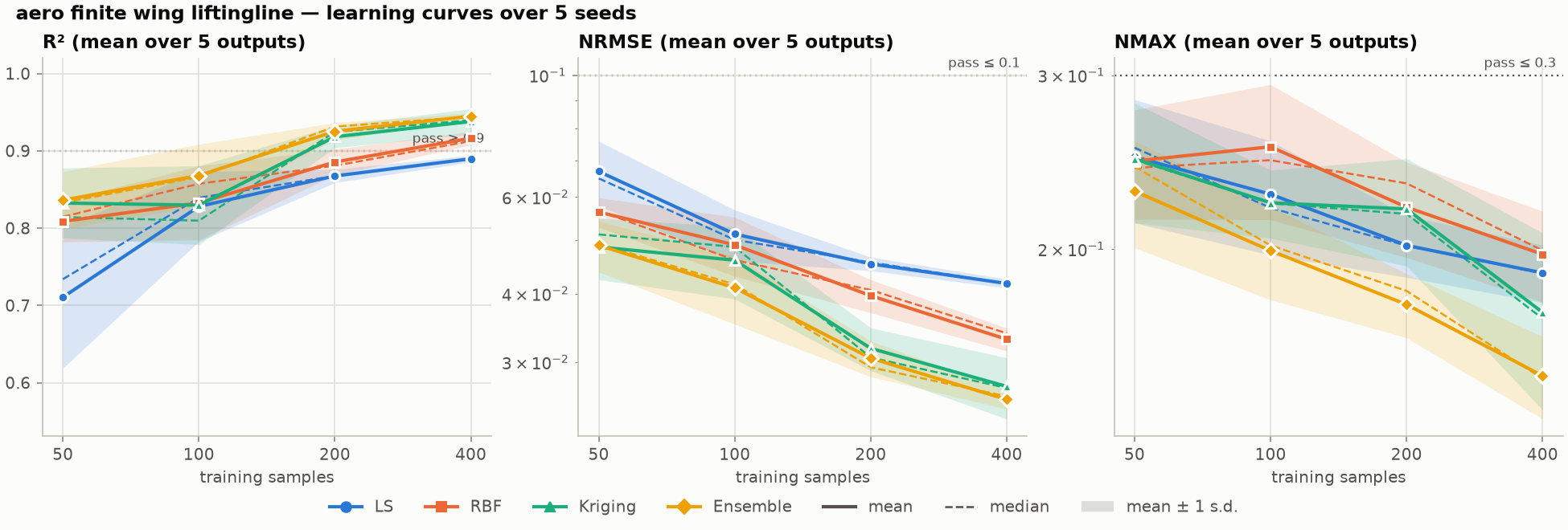
Fig. 13 Finite wing (lifting line).

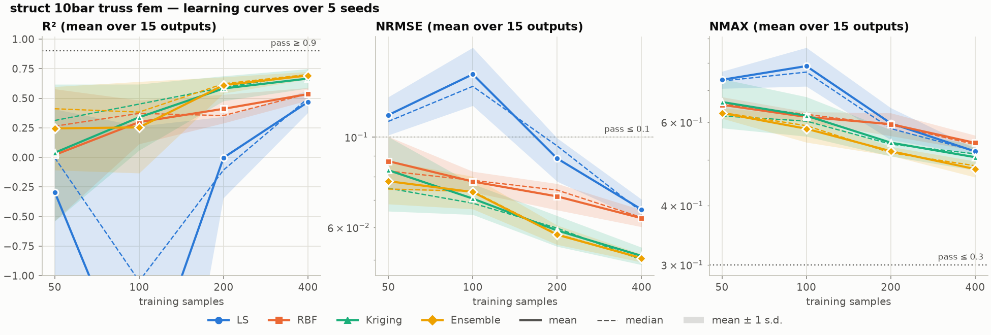
Fig. 14 10-bar truss.

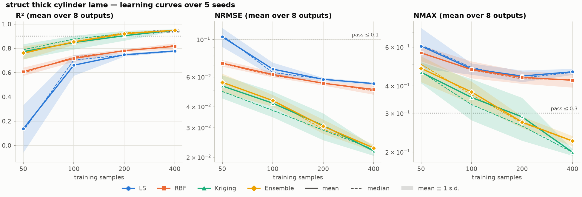
Fig. 15 Thick cylinder.

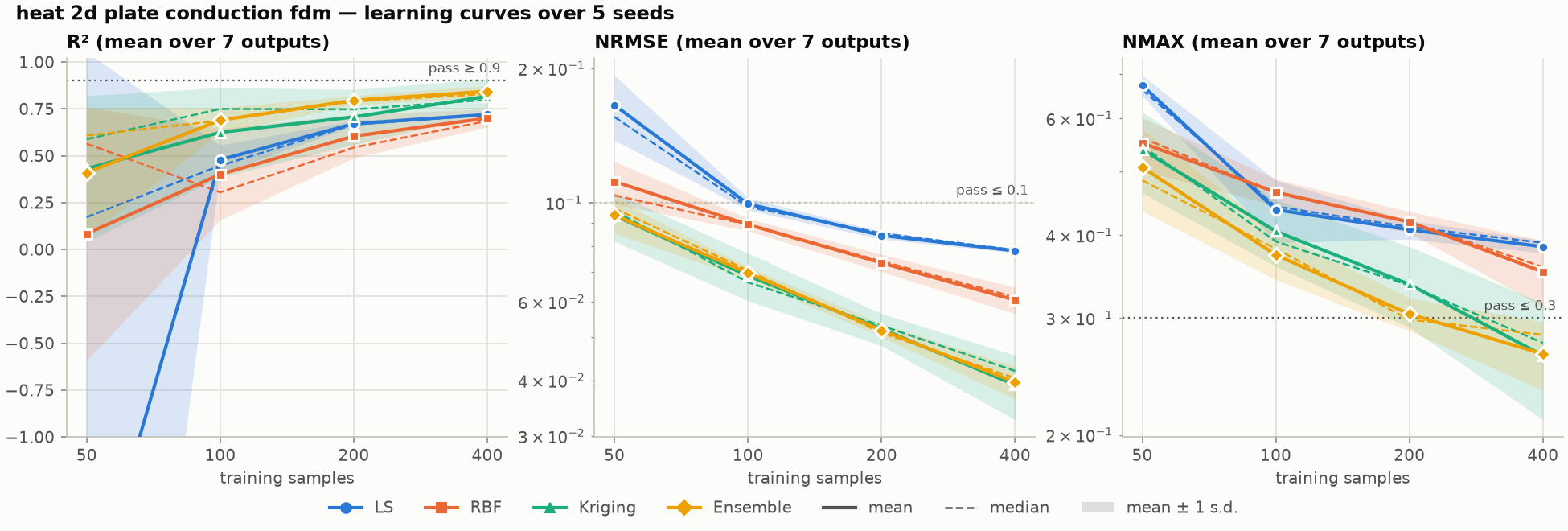
Fig. 16 Plate conduction.

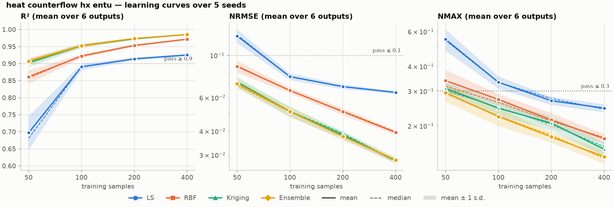
Fig. 17 Counter-flow heat exchanger.

Box plots at \(n = 400\)

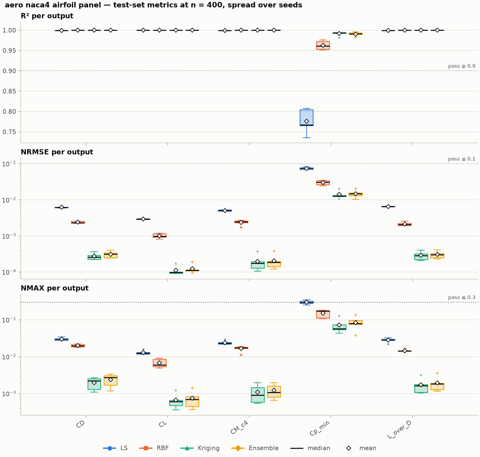
Fig. 18 Airfoil panel method.

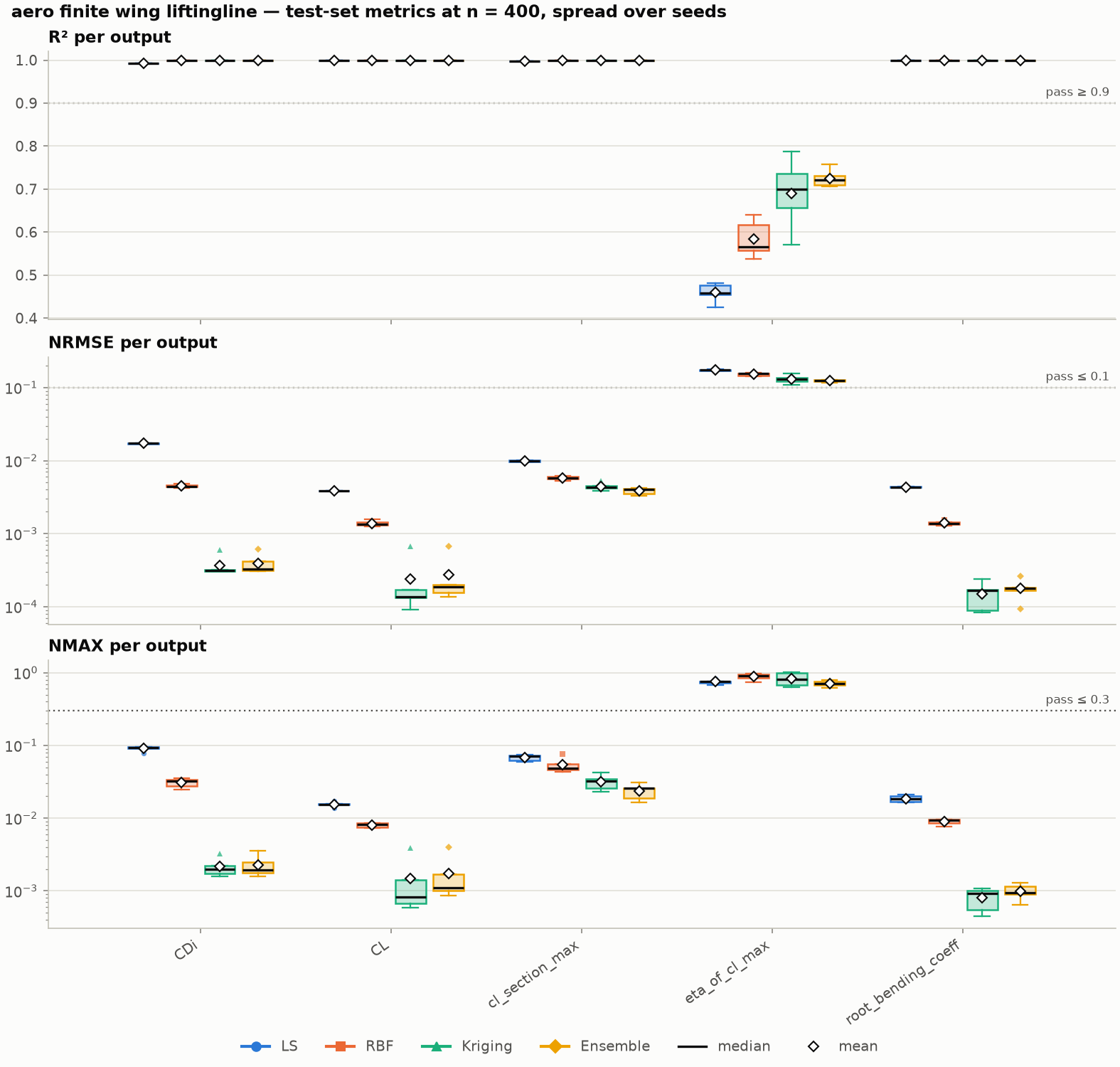
Fig. 19 Finite wing (lifting line).

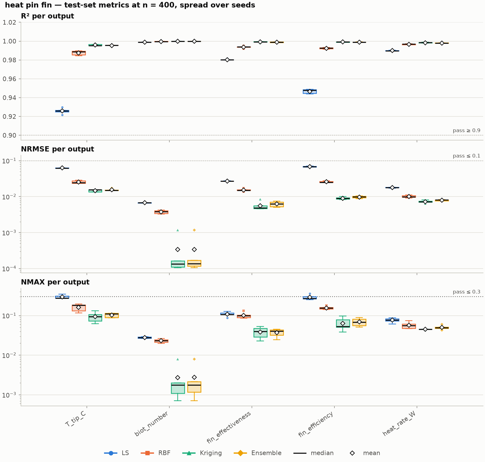
Fig. 20 Pin fin.

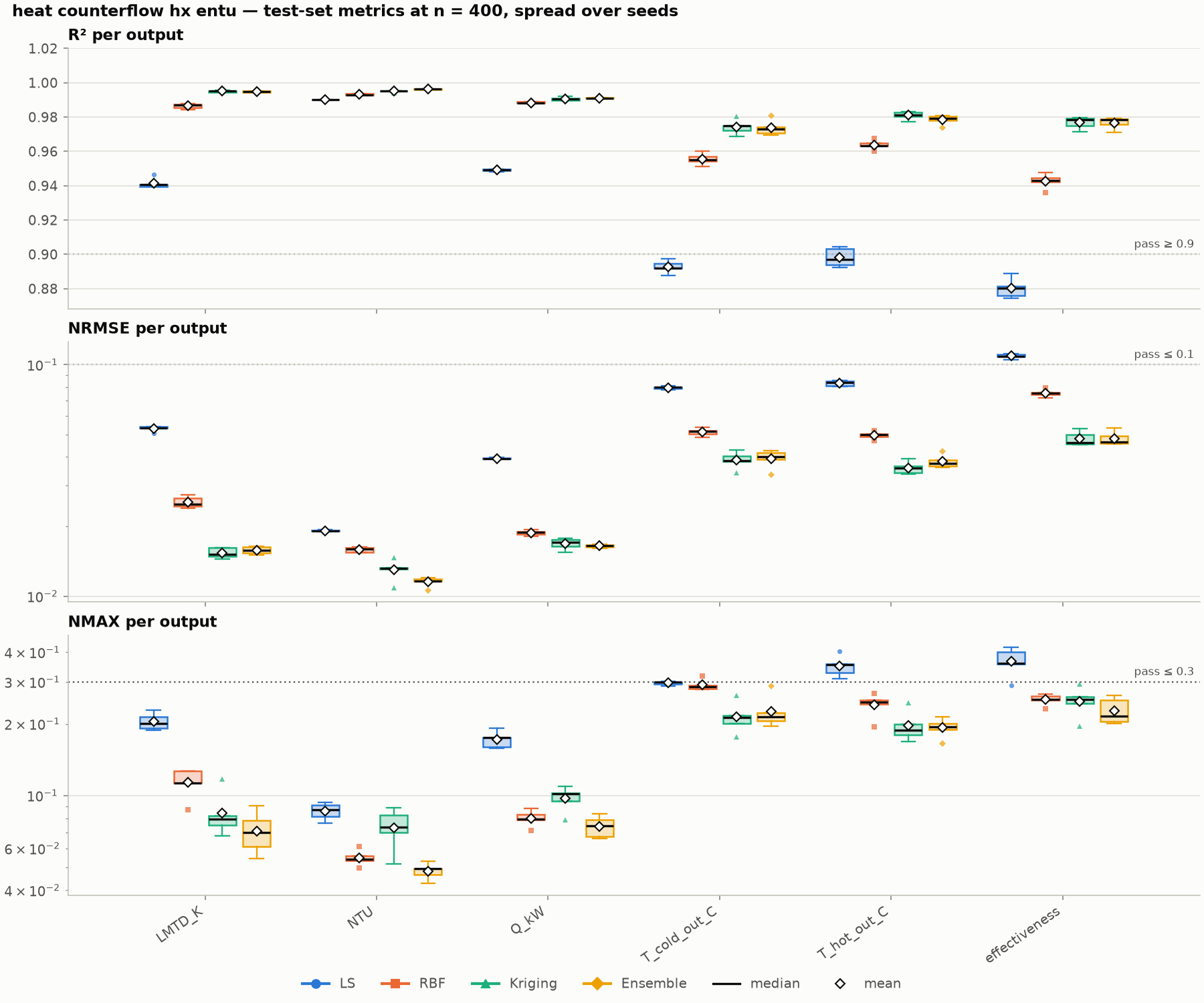
Fig. 21 Counter-flow heat exchanger.